Hi! This is where I write whatever I think needs sharing.
Can you train a text-to-image model without any text?
Despite Betteridge’s law, I contend the answer is “probably”. I’d prefer to be writing a post without a question mark at the end of the title, but I haven’t actually gotten it to work yet. This post is something of a research log documenting my efforts, though written ex post. This code for the models and data processing is here.
Why should it be possible?
A text-to-image model is one which, well, takes in text and outputs images. DALL-E and Midjourney are the most famous examples, but there are tons. The user types in a prompt (“Central Park during the freak snowstorm of 2024, shot on Hasselblad medium format”) and the model generates an image that resembles the prompt. They’re trained on pairs of captions and images, so the objective is more like an image that would have that caption. The modern wave was kicked off by DALL-E and to a greater extent CLIP. Most of the open source models I’ve seen exploit CLIP in some way, and the proprietary ones probably do too. It should, in my opinion, be possible to use CLIP and an unlabeled set of images to make a text-to-image model.
CLIP was released back in January 2021. It’s a model that associates images and captions. Both images and captions are projected into a shared vector space and the training objective is to maximize the cosine similarity between images and their captions1. This training objective, plus lots of data and compute, results in a model that knows a ton about images. It can identify locations, famous people, objects, animals, and do them in combination. This web app lets you search the LAION-5B dataset using CLIP. It’s unfortunately down right now, but maybe you’ll be lucky and it’ll be up when you read this. As an illustration of the power of CLIP, the results will dramatically change if you tack “shot with Sony a7R” (or some other camera) onto the end of a query that returns photos. People who label their photos with what type of camera they used take different types of photos from people who don’t, and people who use different cameras take different types of photos from each other. CLIP knows this. And it works for image to image comparisons as well - a picture of the Golden Gate Bridge’s embedding will have high cosine similarity to other pictures of the Golden Gate, regardless of angle, weather, time of day, etc. Even paintings and drawings will match.
So, since CLIP knows what labels go with which images, you shouldn’t need labels of your own to train a text-to-image model. You should be able to entirely rely on CLIP for the supervision. That’s the goal.
A baseline
My first attempt simply conditioned image generation on the CLIP embeddings of the images. This works, you can input an image(’s embedding) and get a similar image out. The model learns the inverse of CLIP’s image projection function. But if you input a text embedding instead, things are not so rosy.
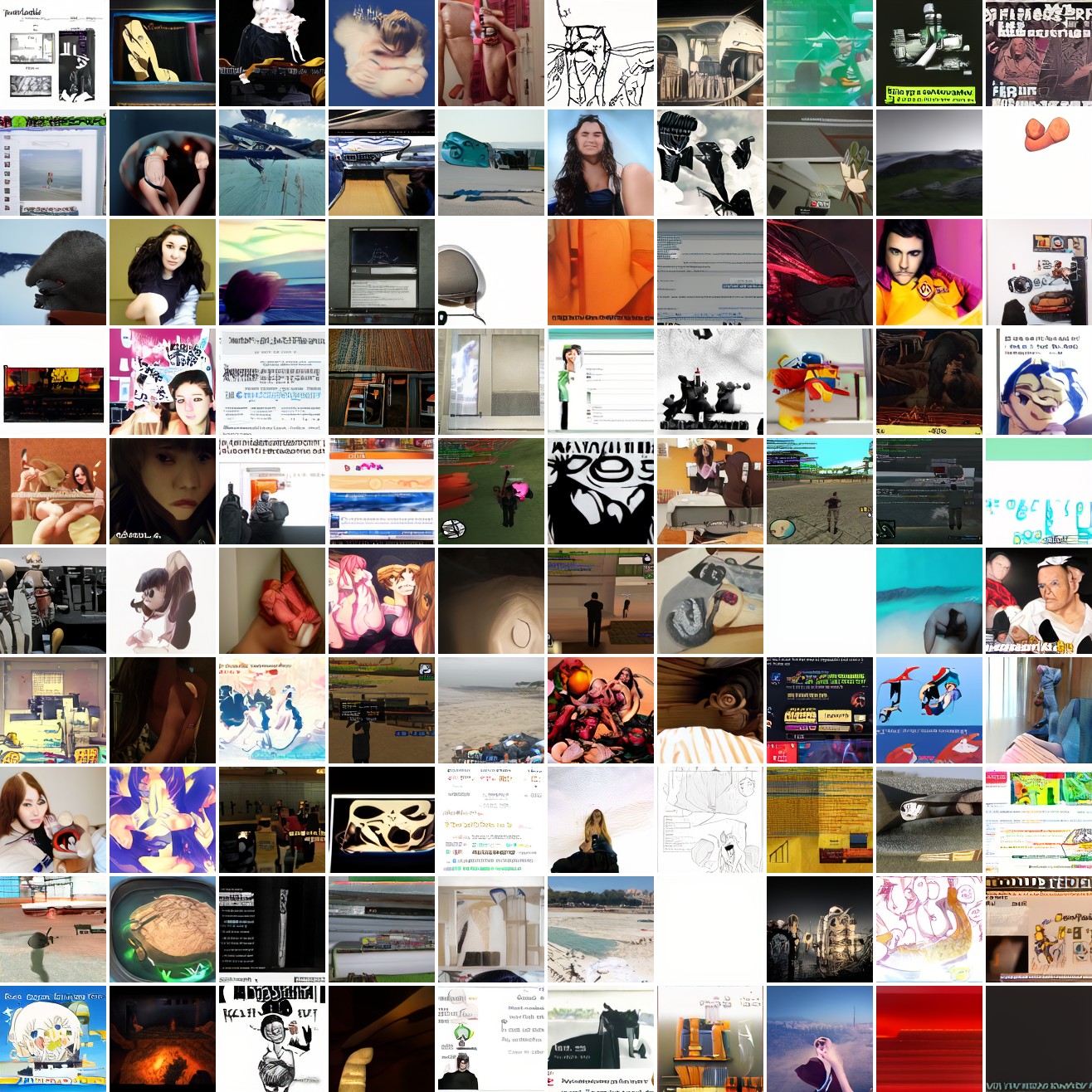
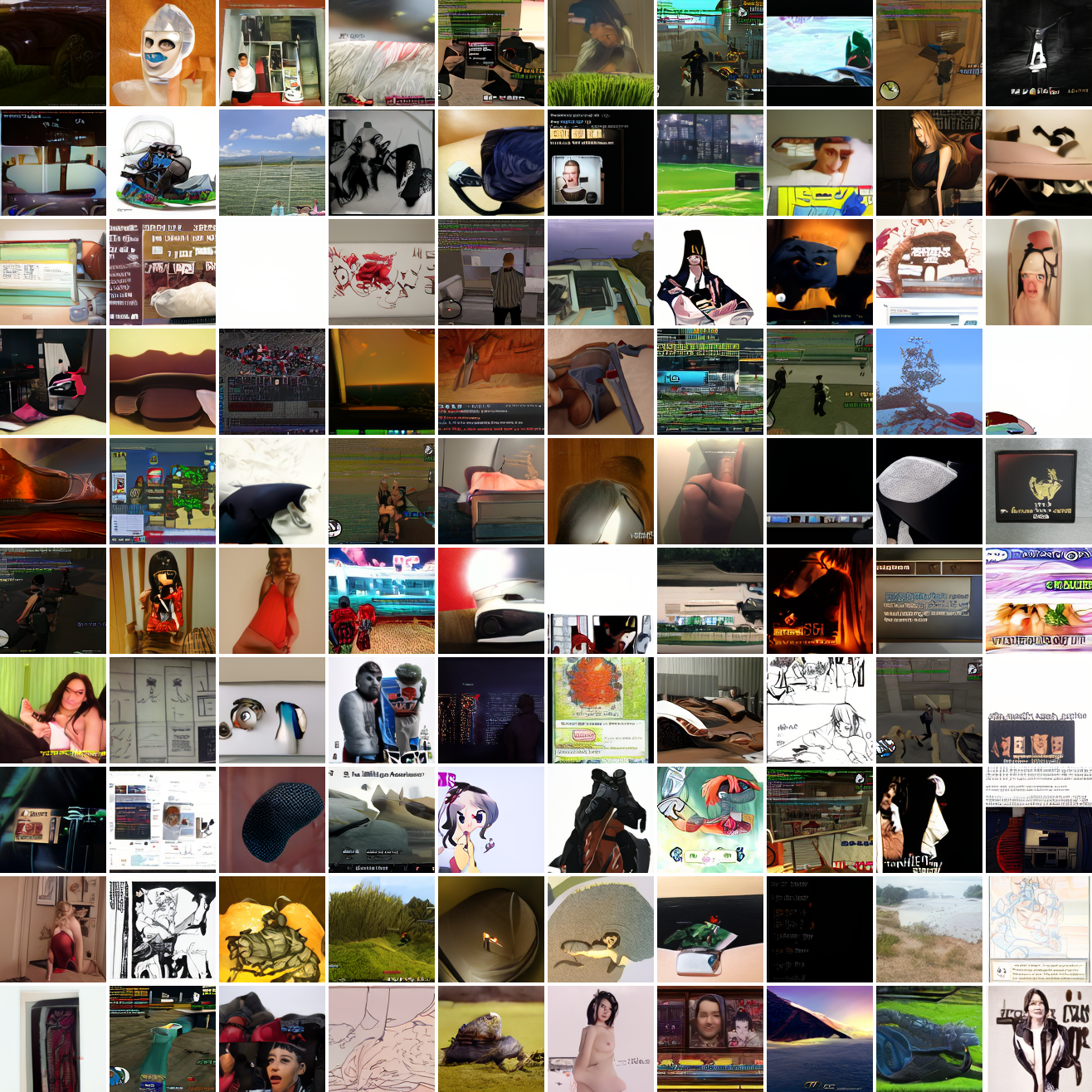
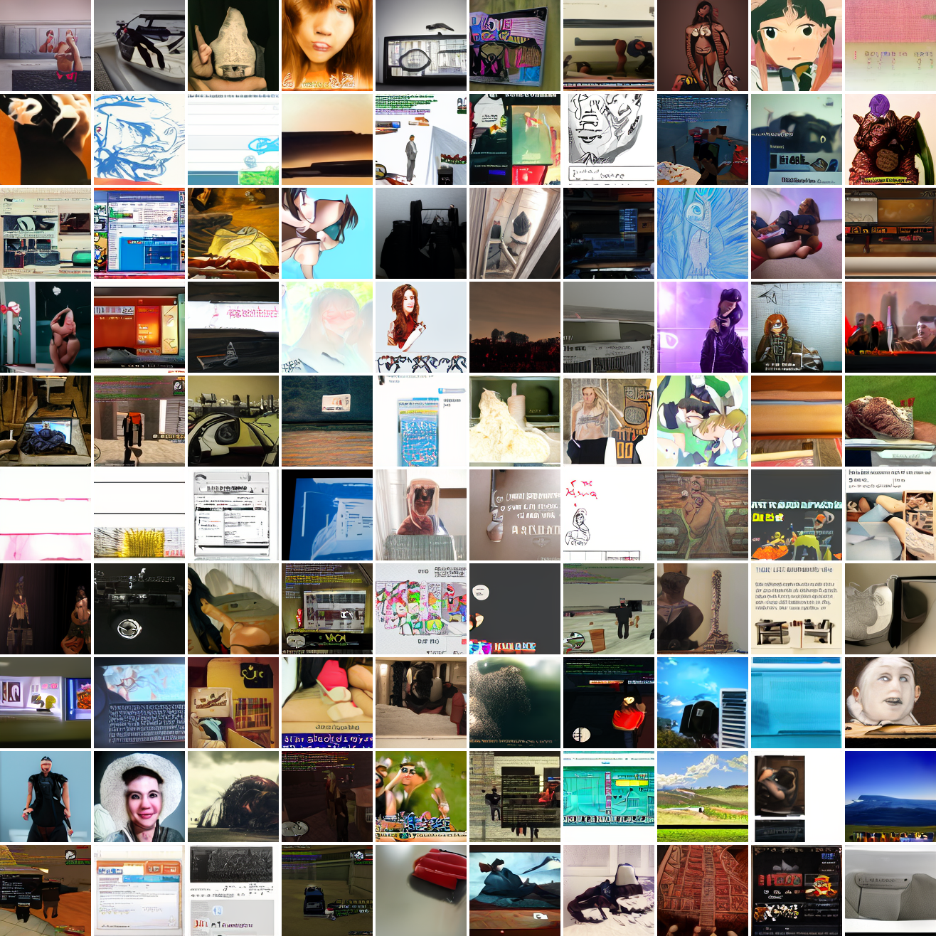
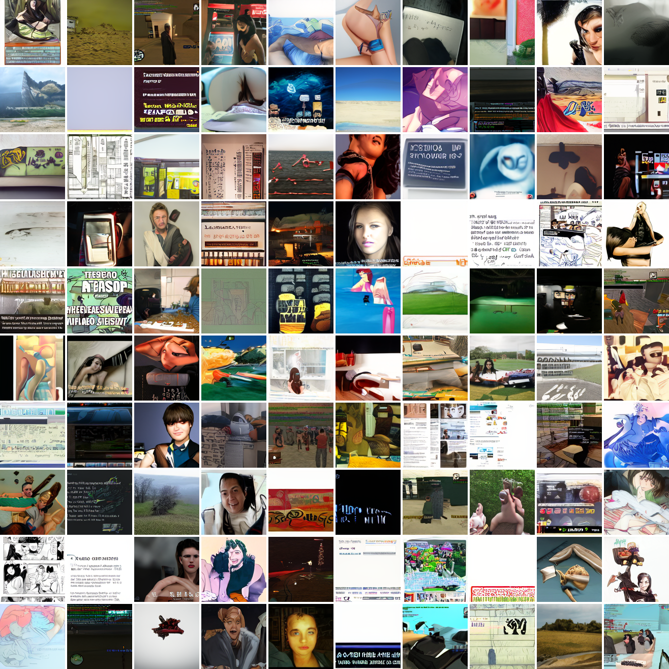
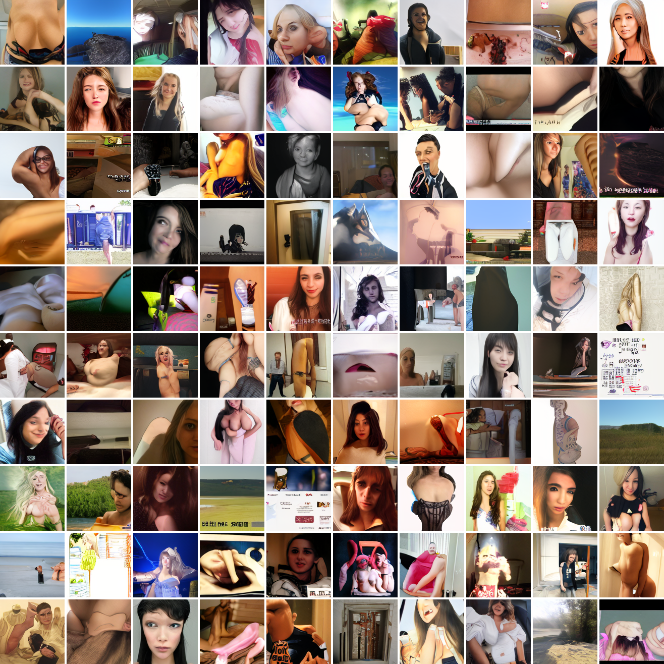
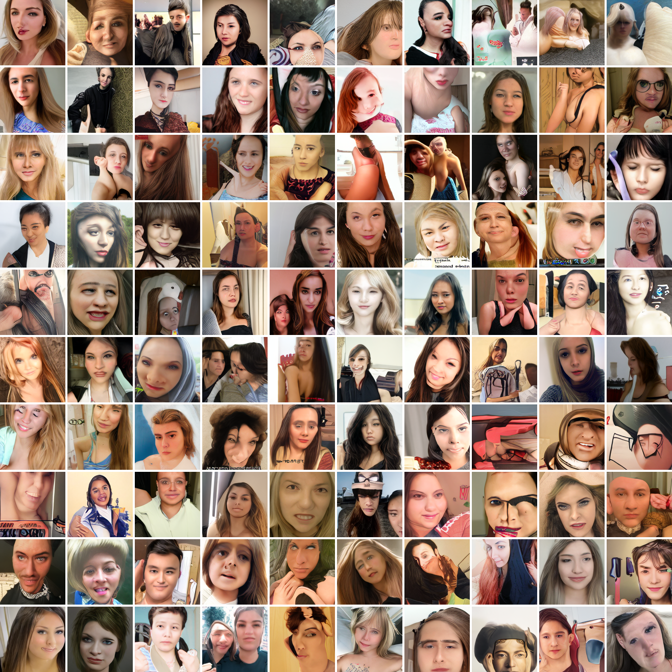
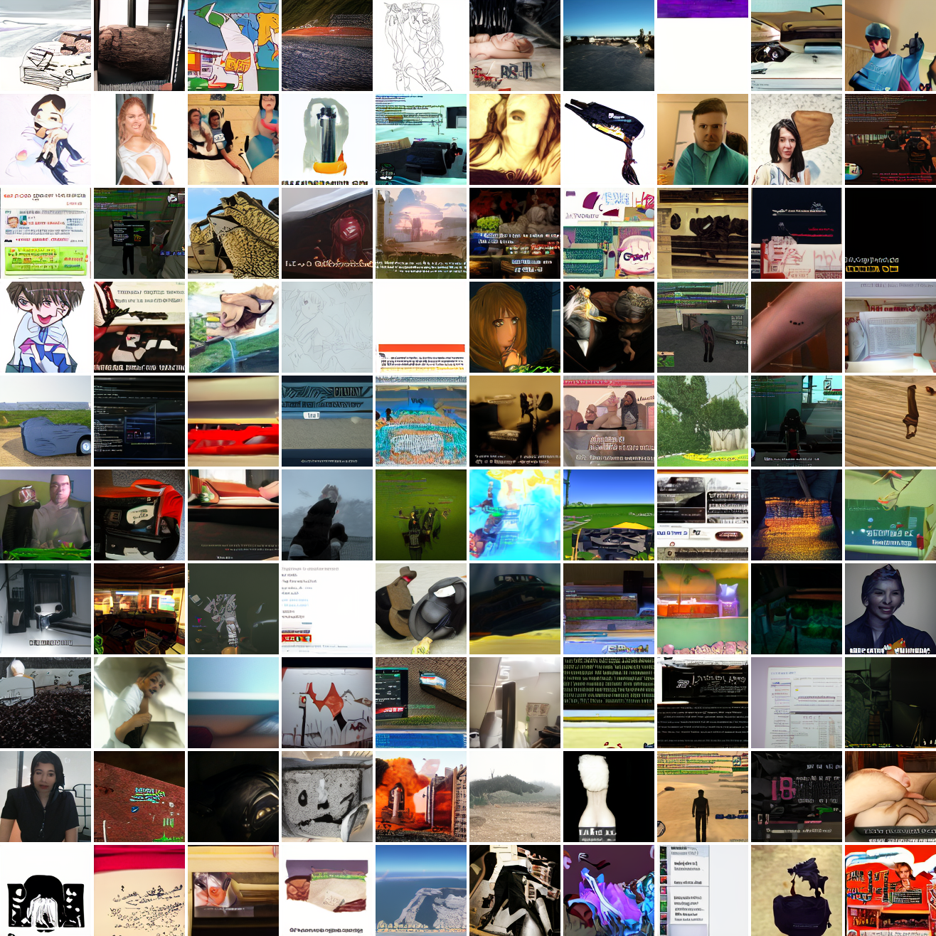
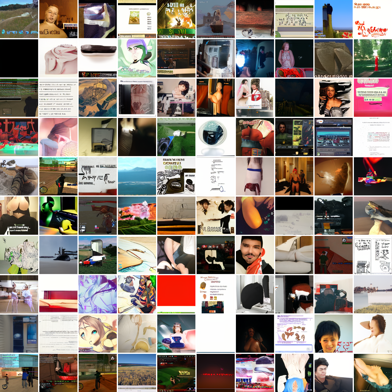
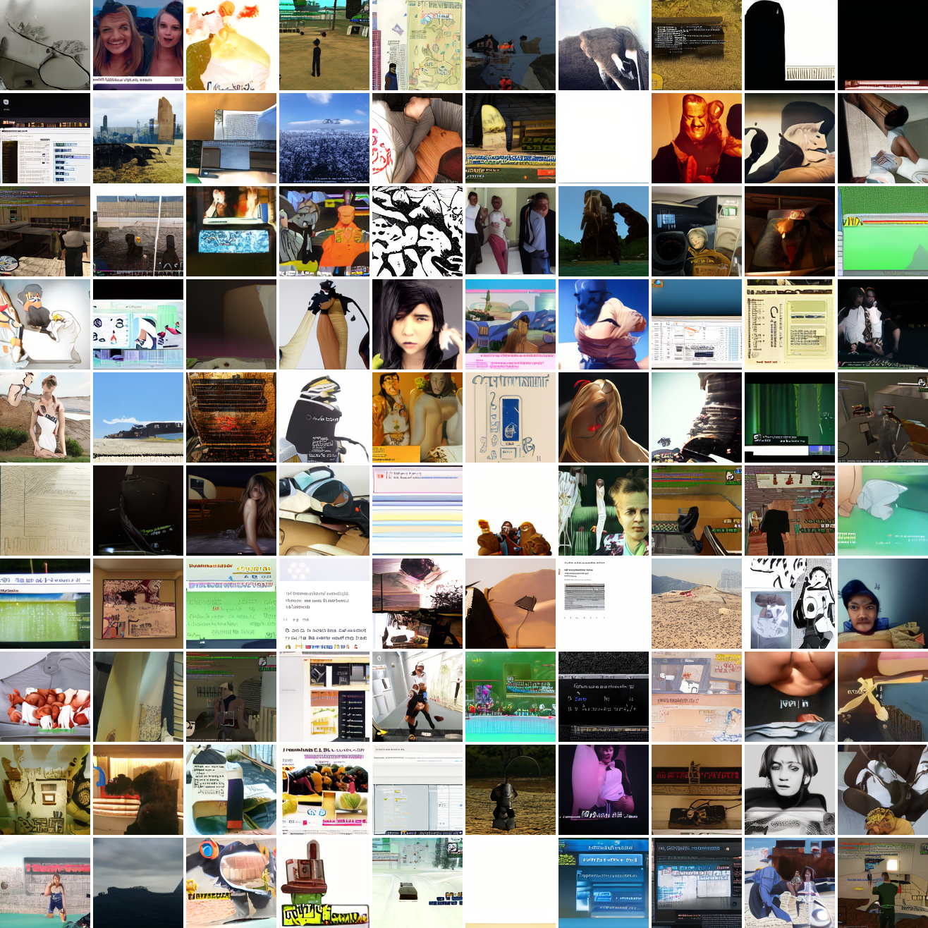
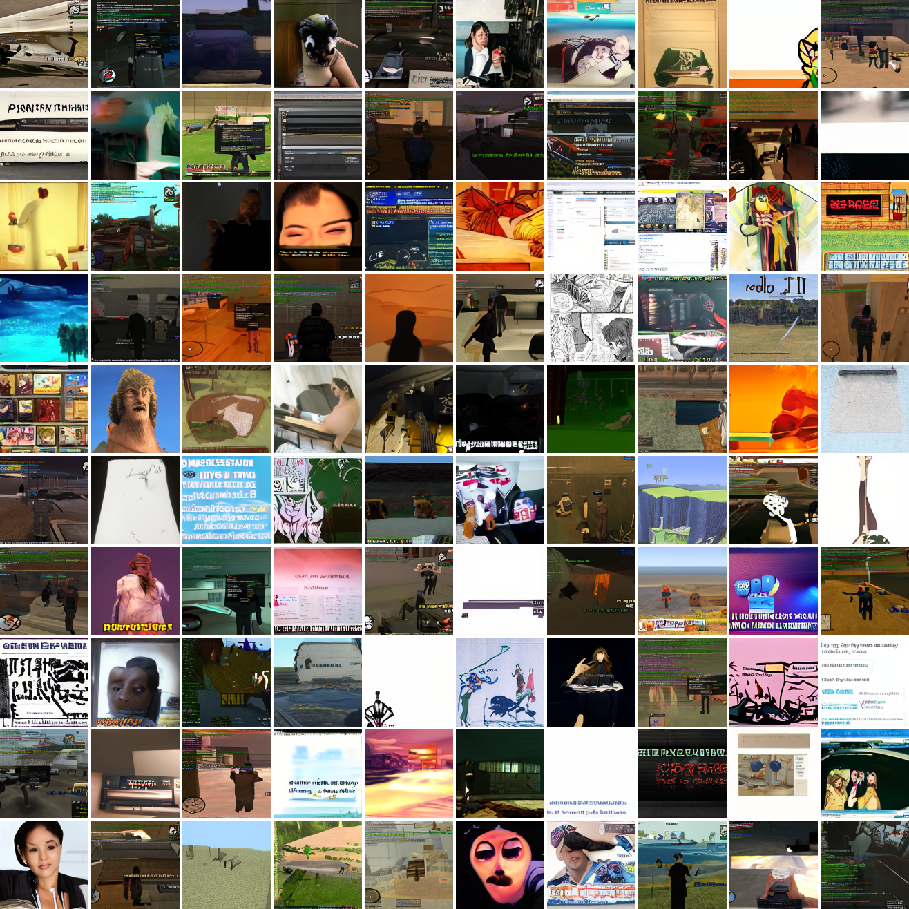
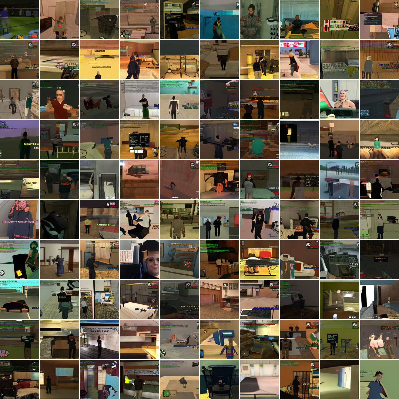
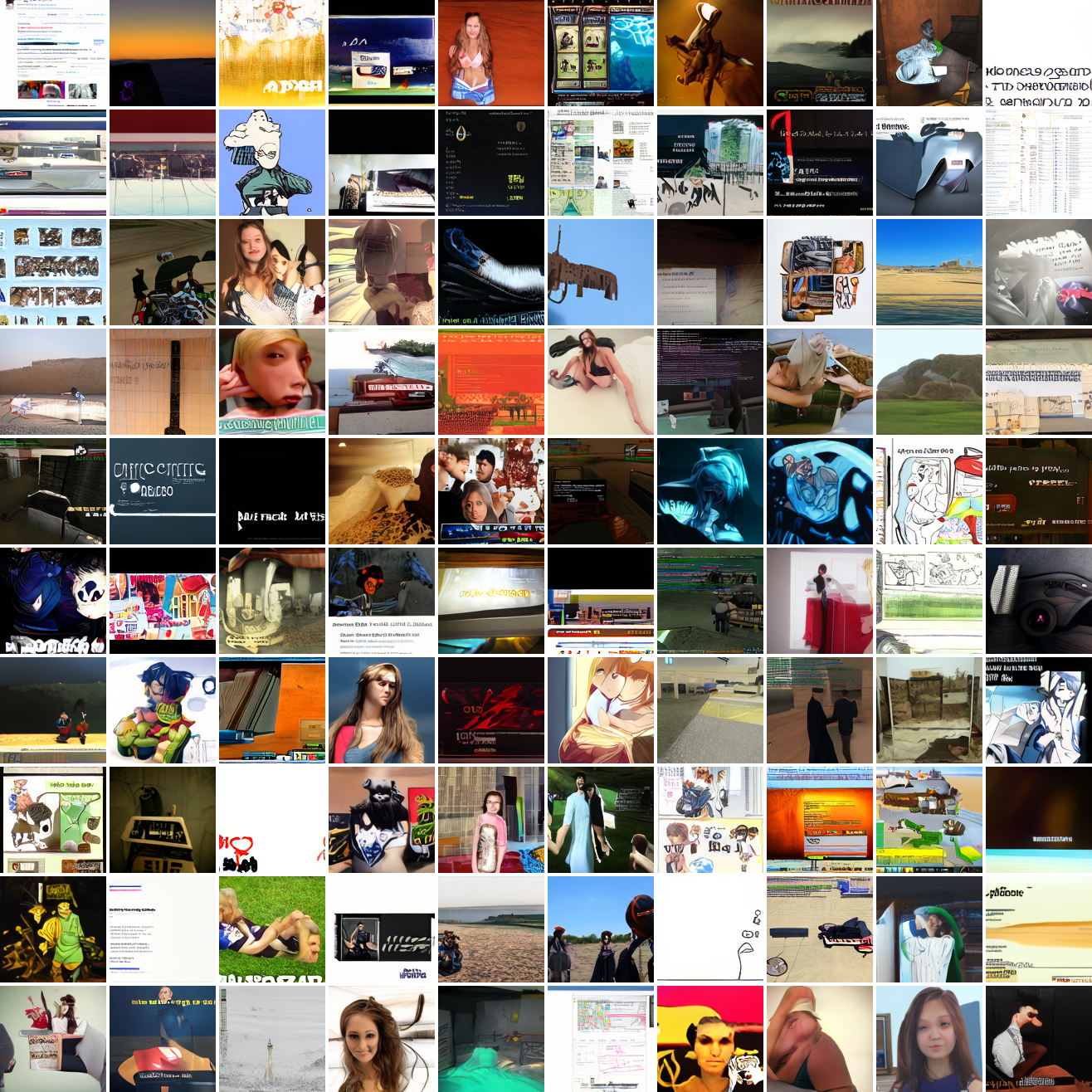
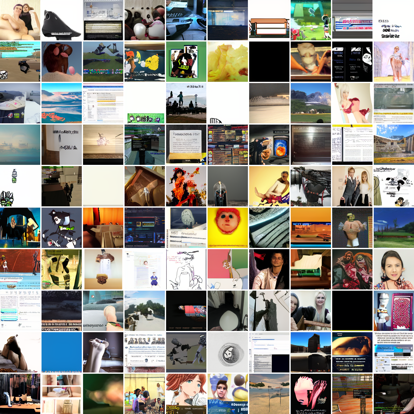
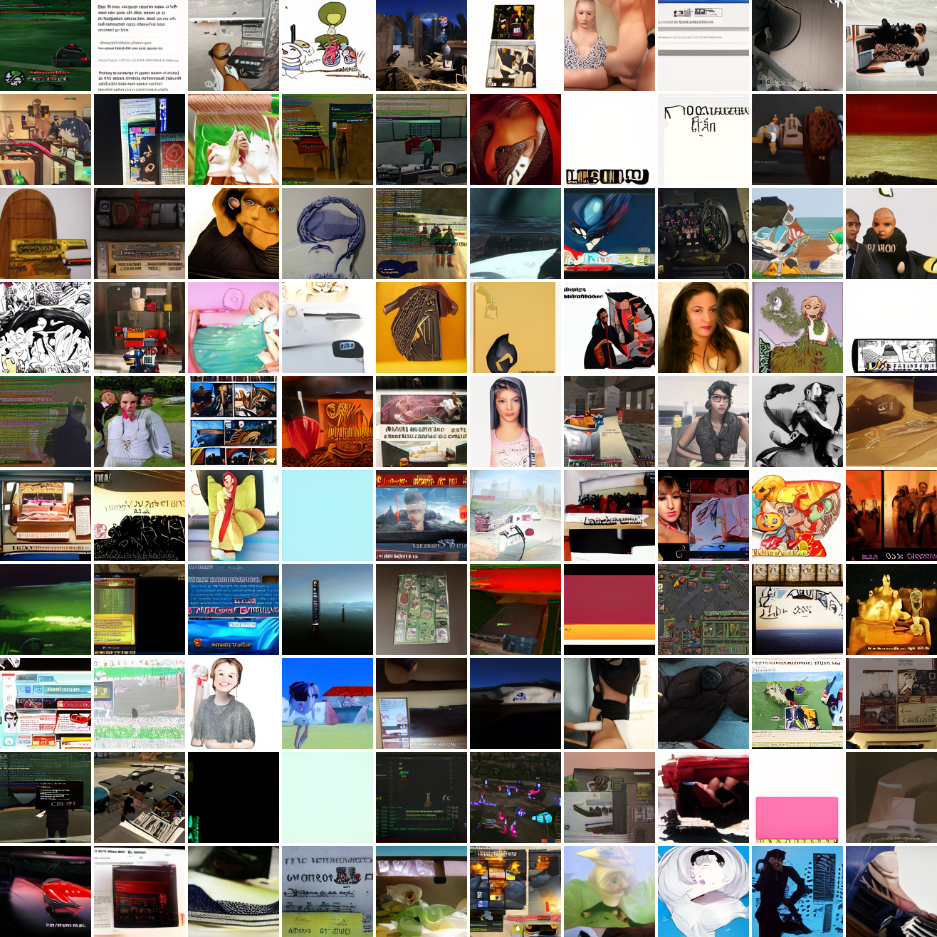
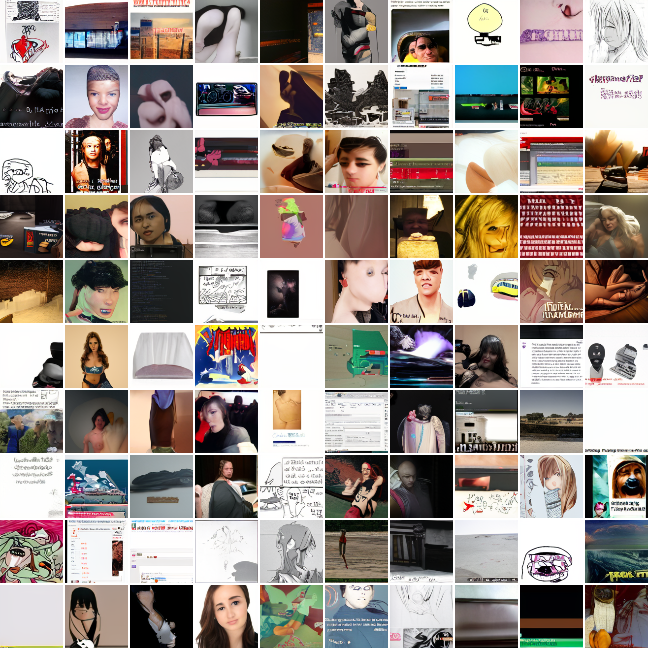
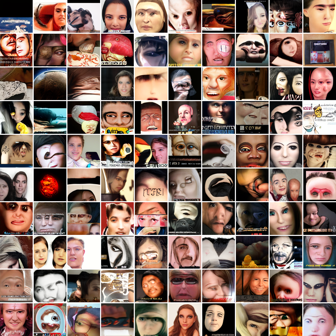
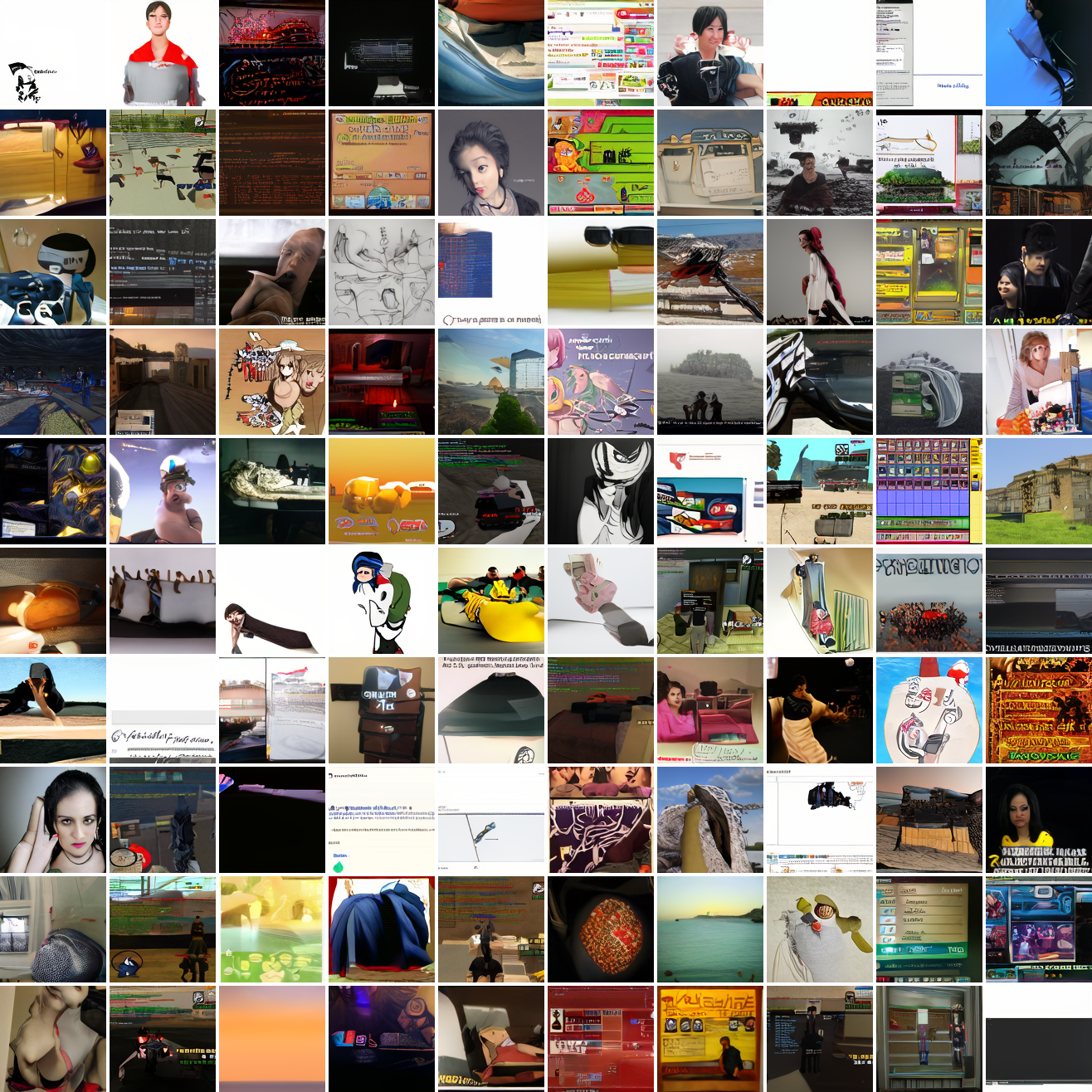
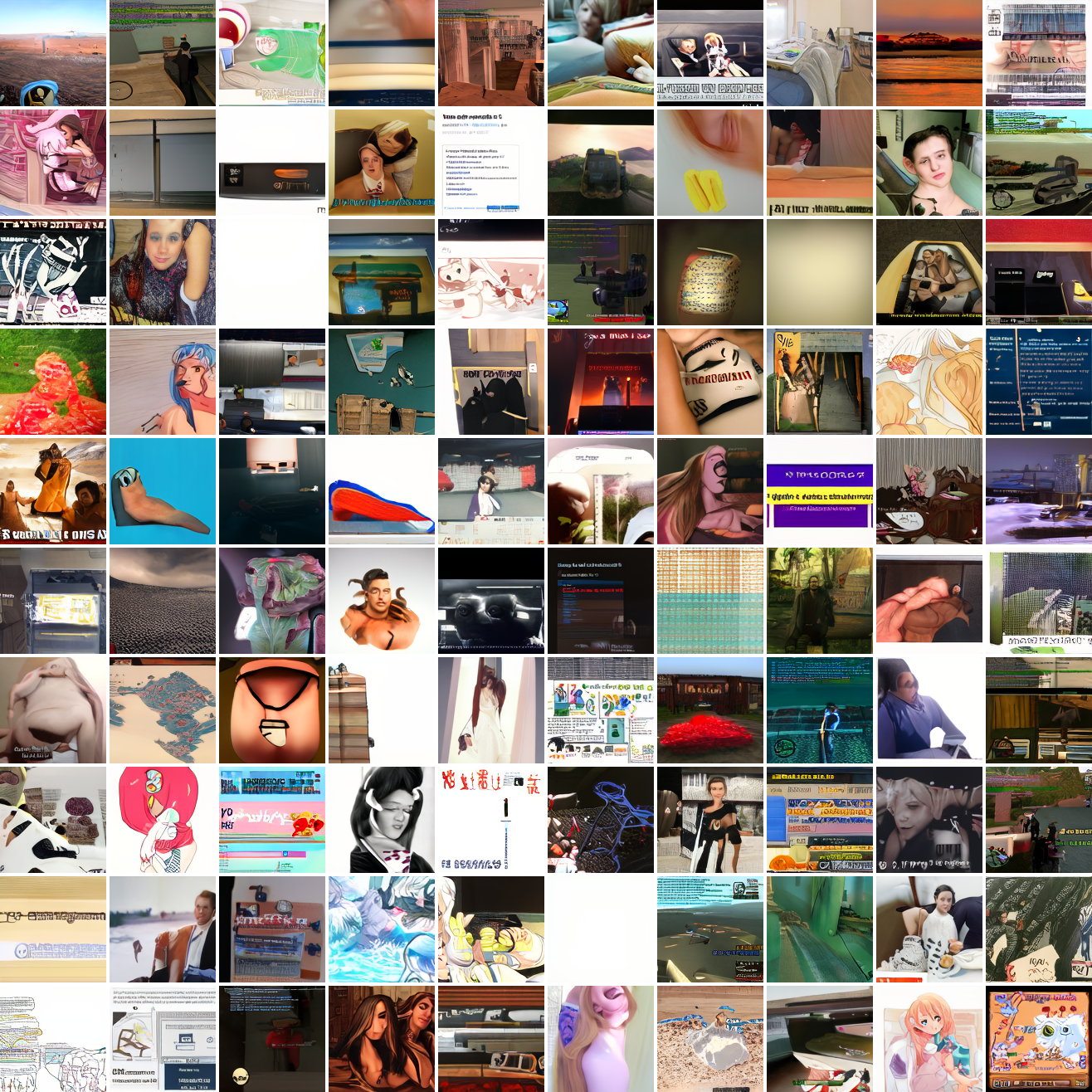
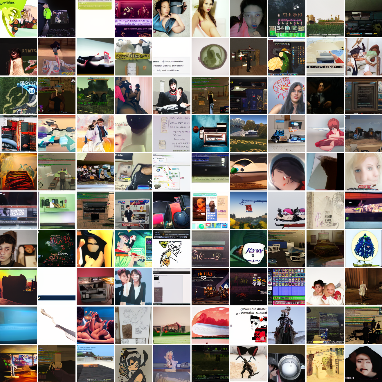
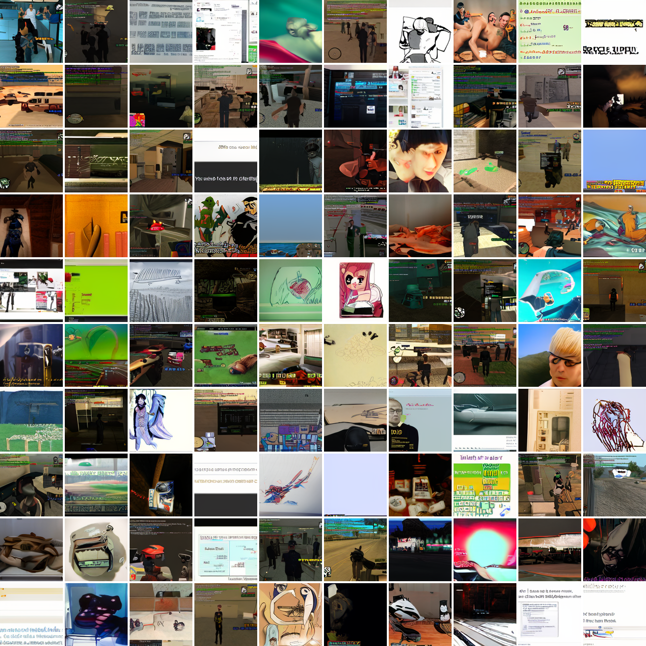
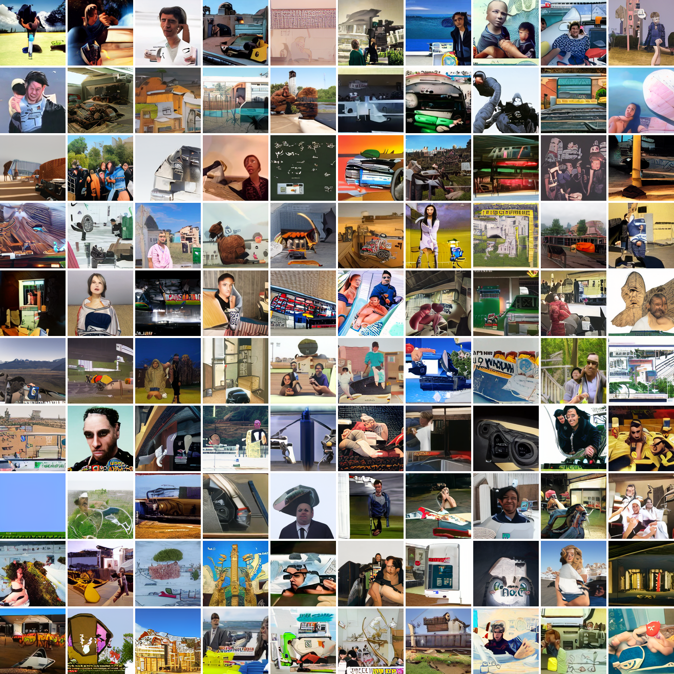
Here’s 100 samples from the baseline model conditioned on a photo of a friend of mine. In the photo she has a sideshave, with the hair on her left side shaved and the hair on her right long. I think that’s why so many of the samples have the head tilted to the model’s right. She’s also wearing glasses in the prompt image, which is why so many of the samples have glasses.
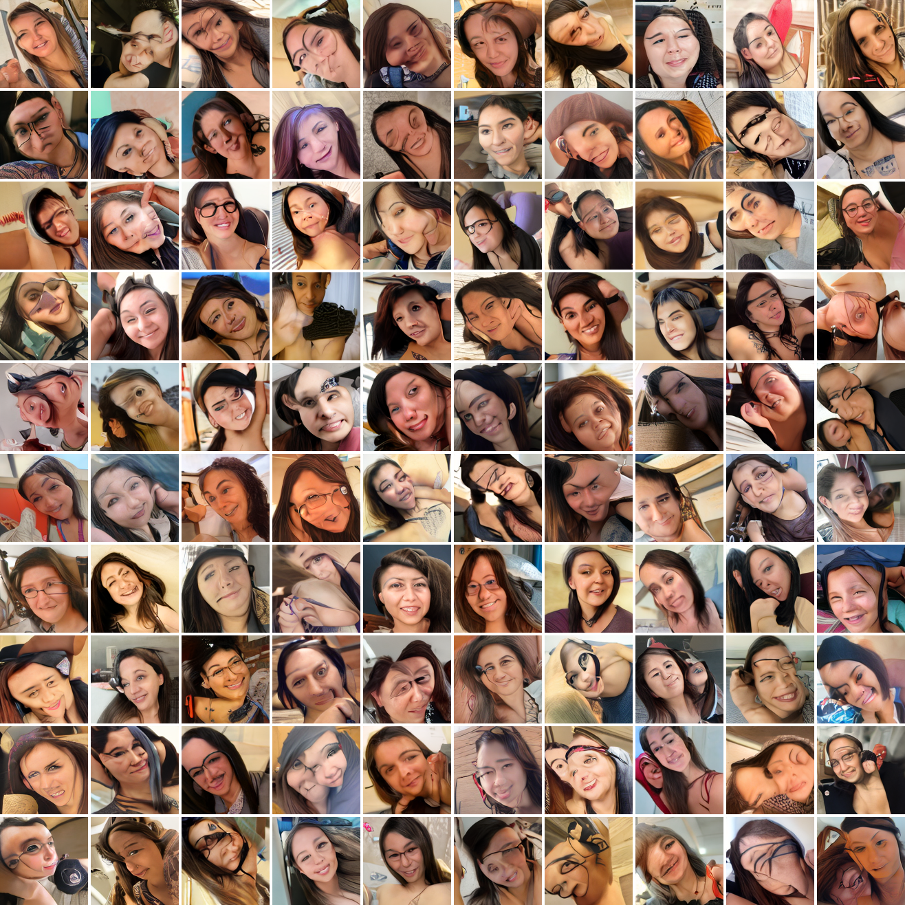
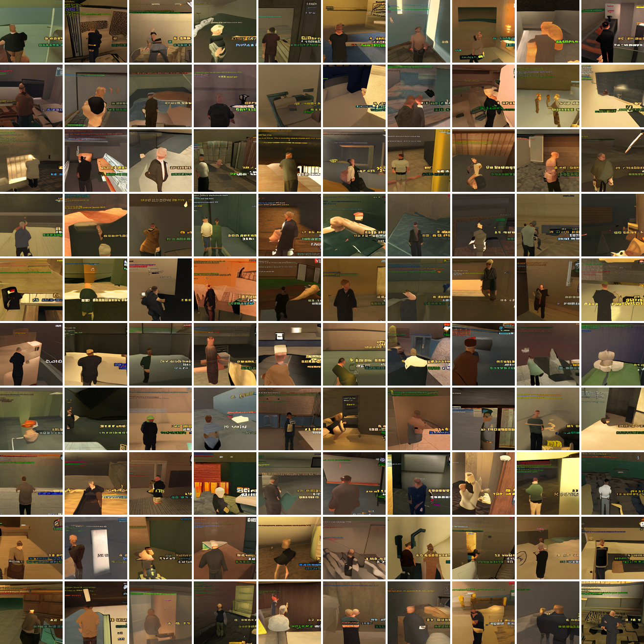
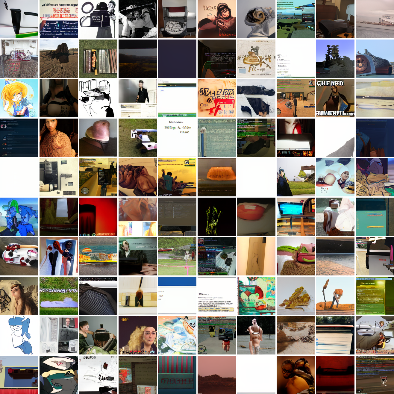
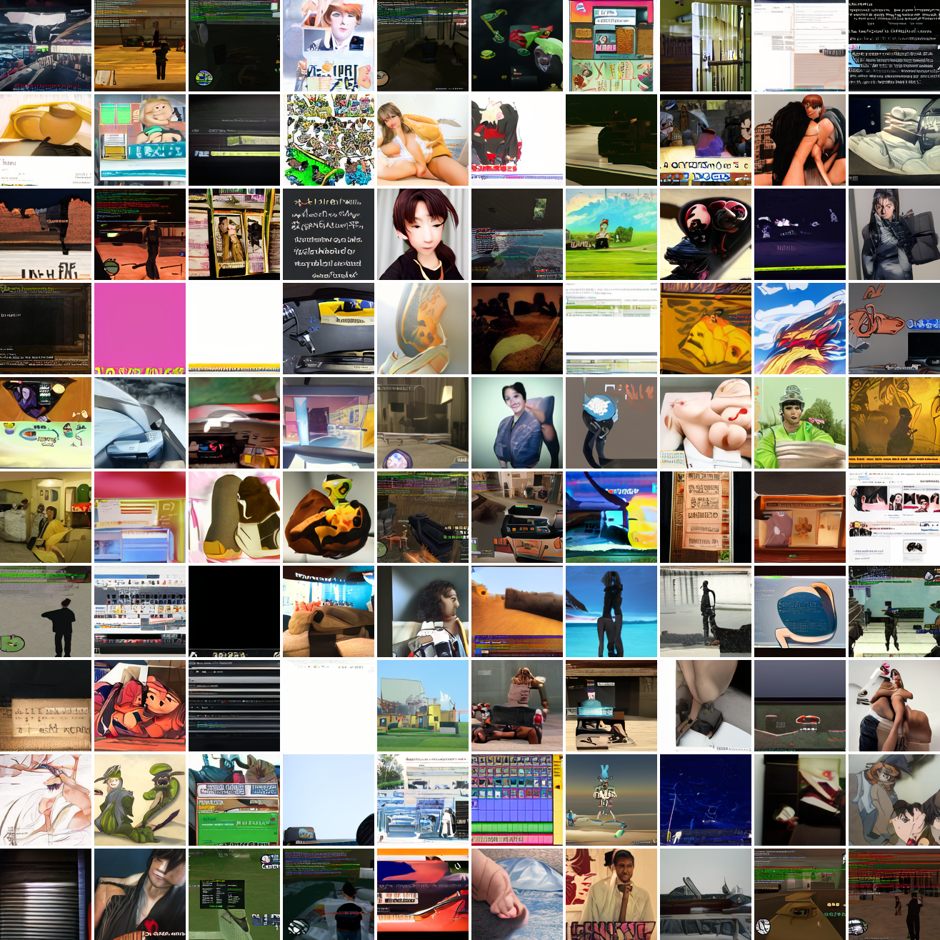
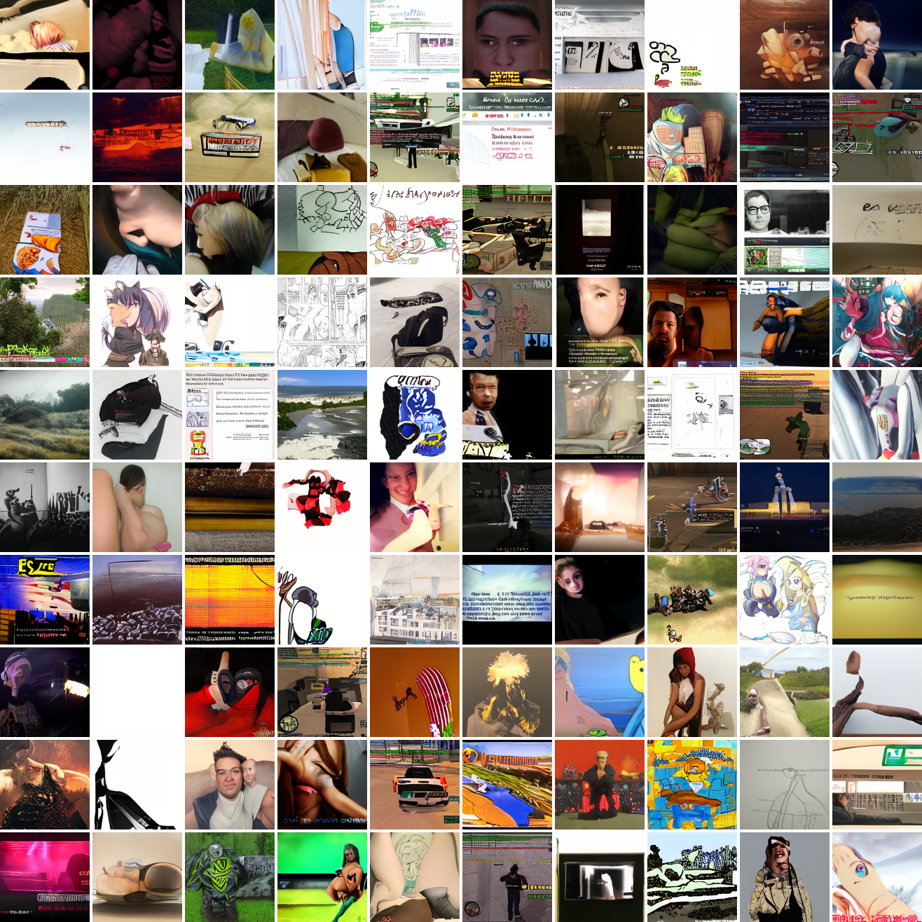
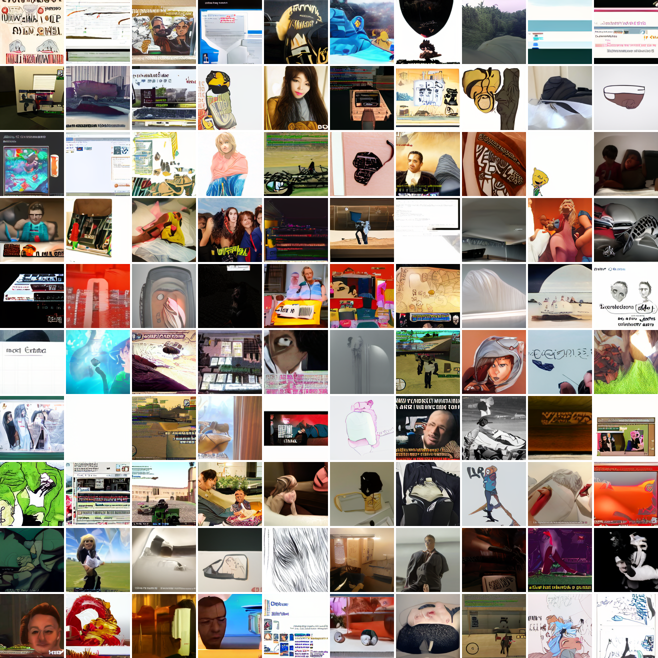
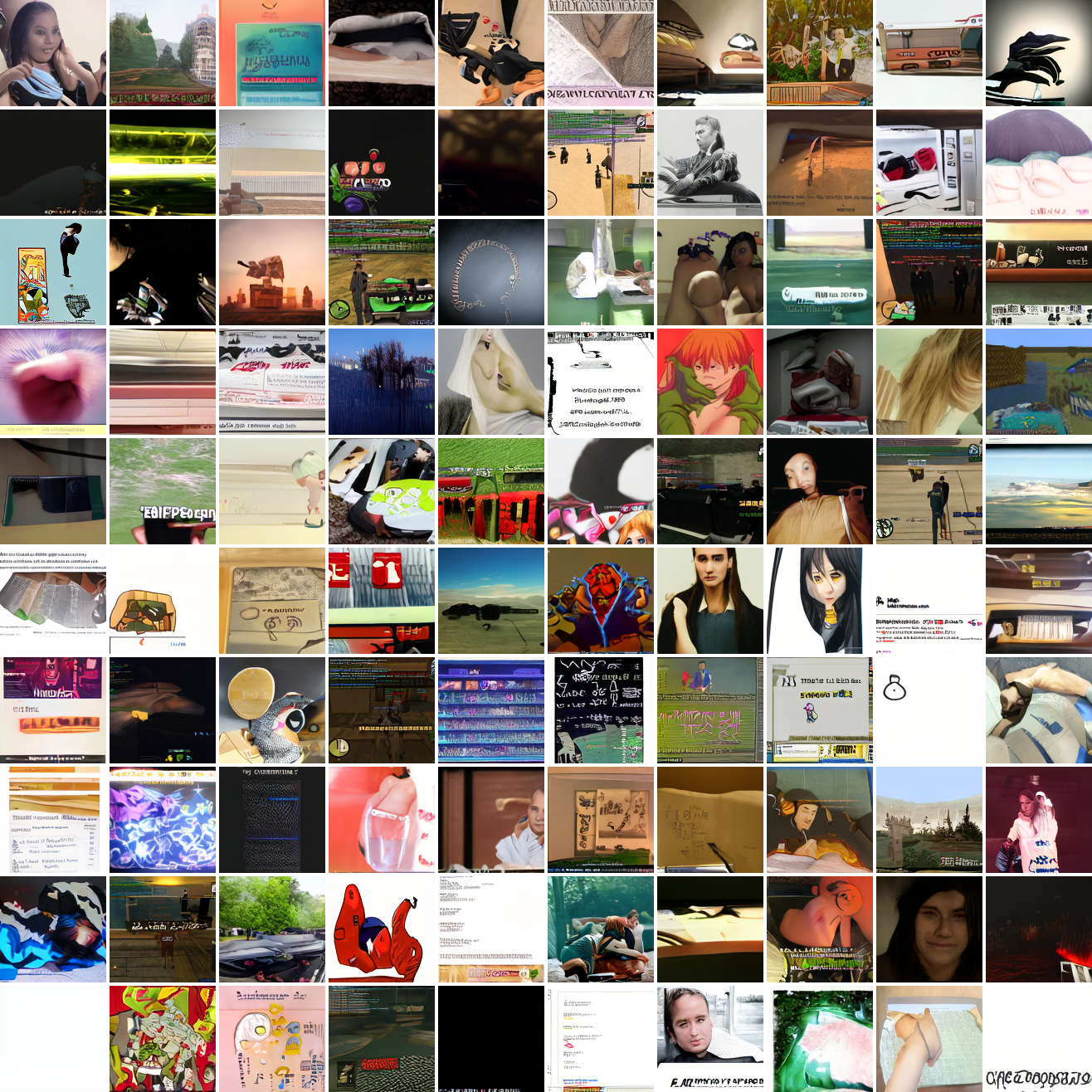
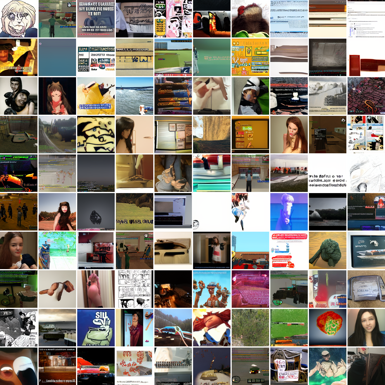
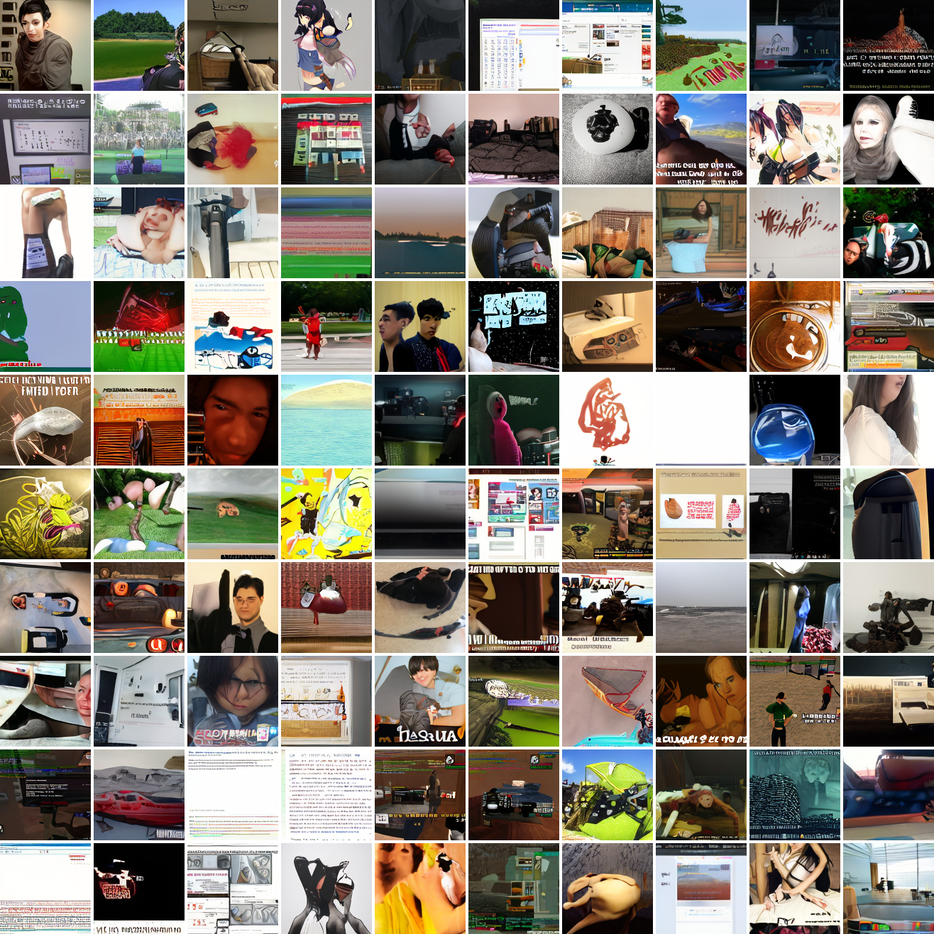
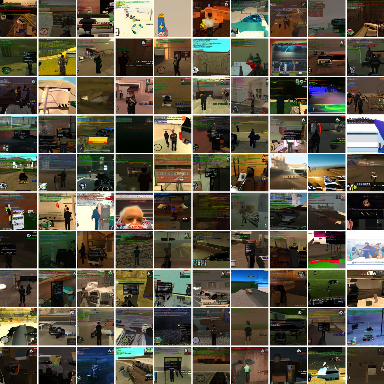
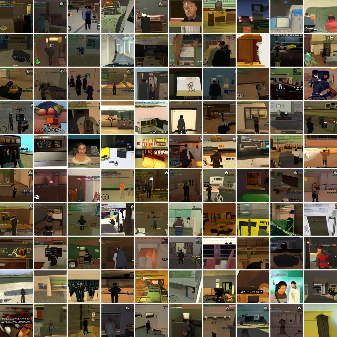
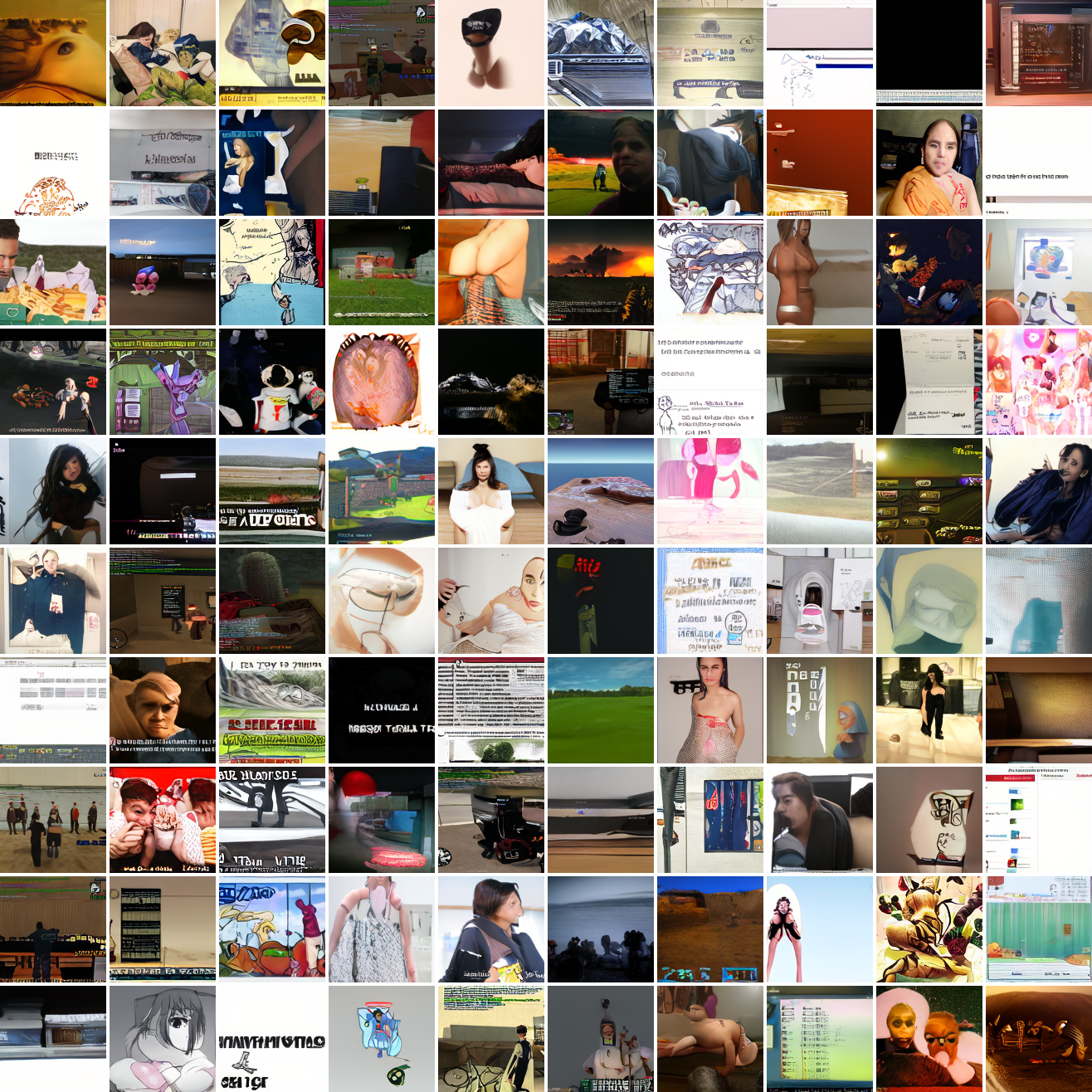
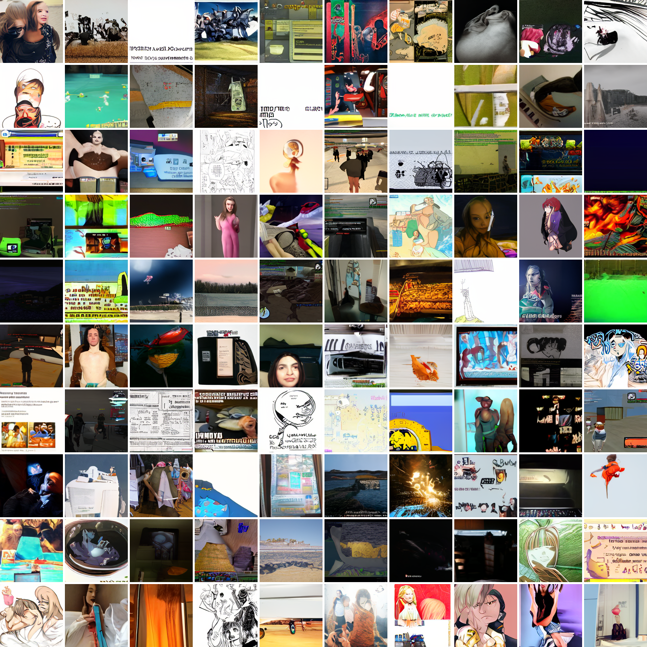
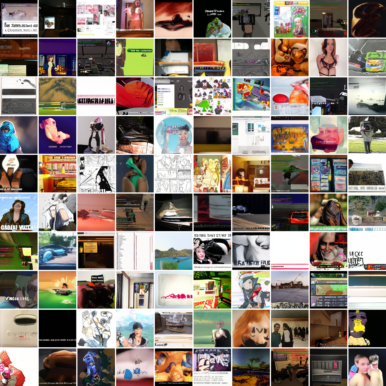
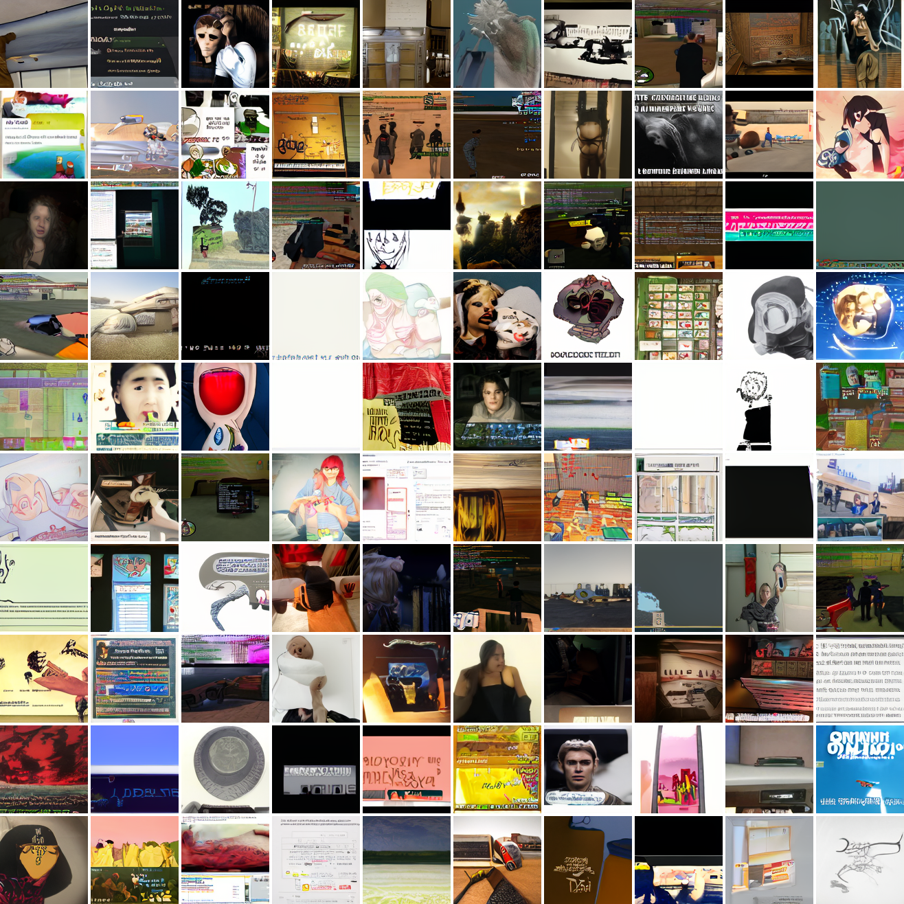
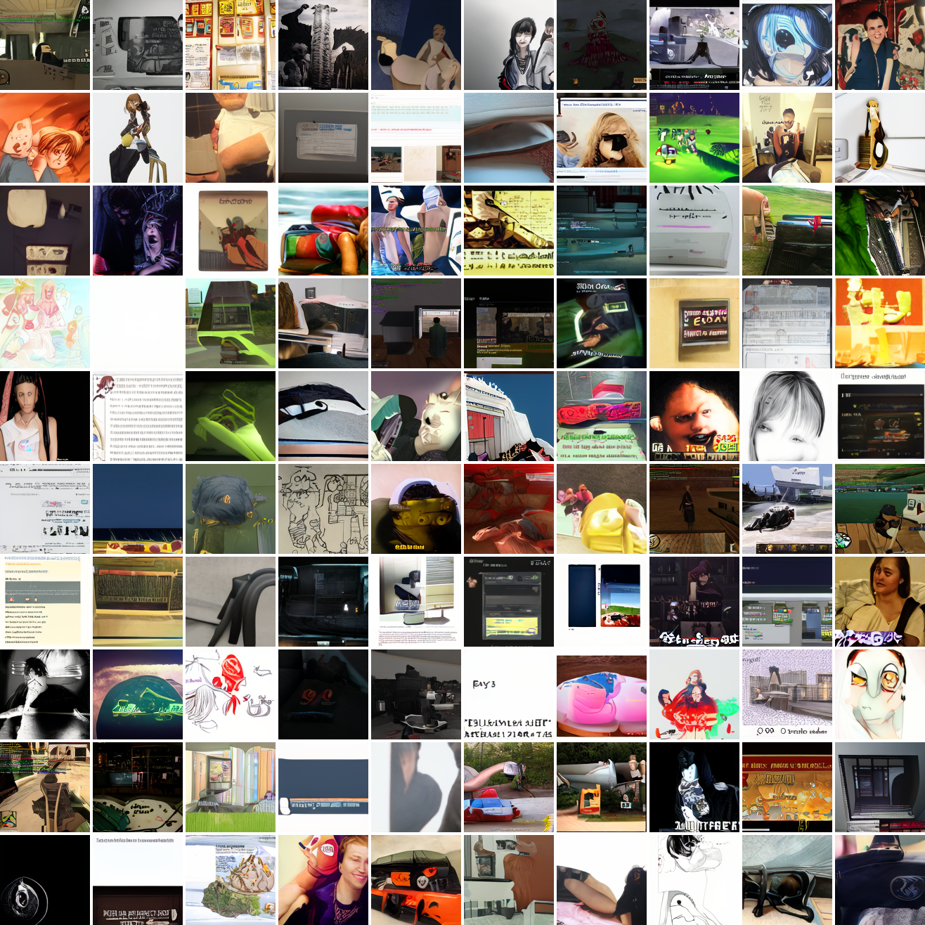
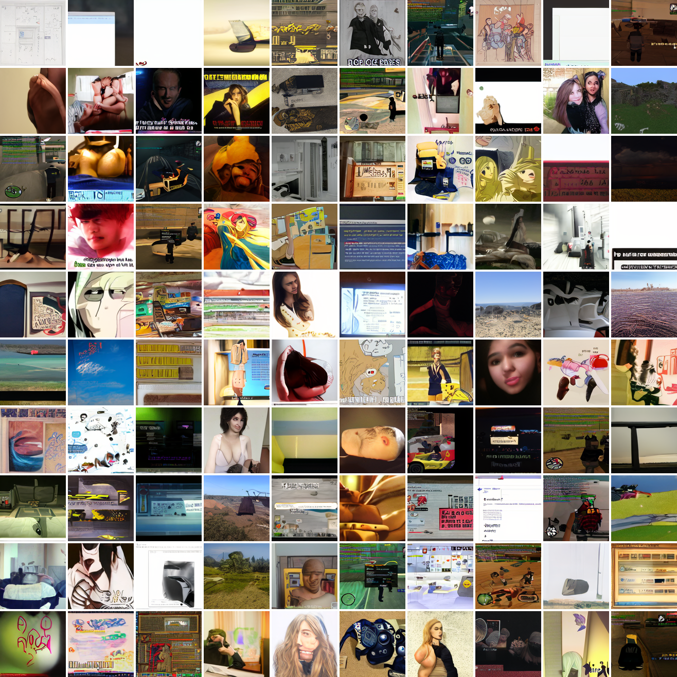
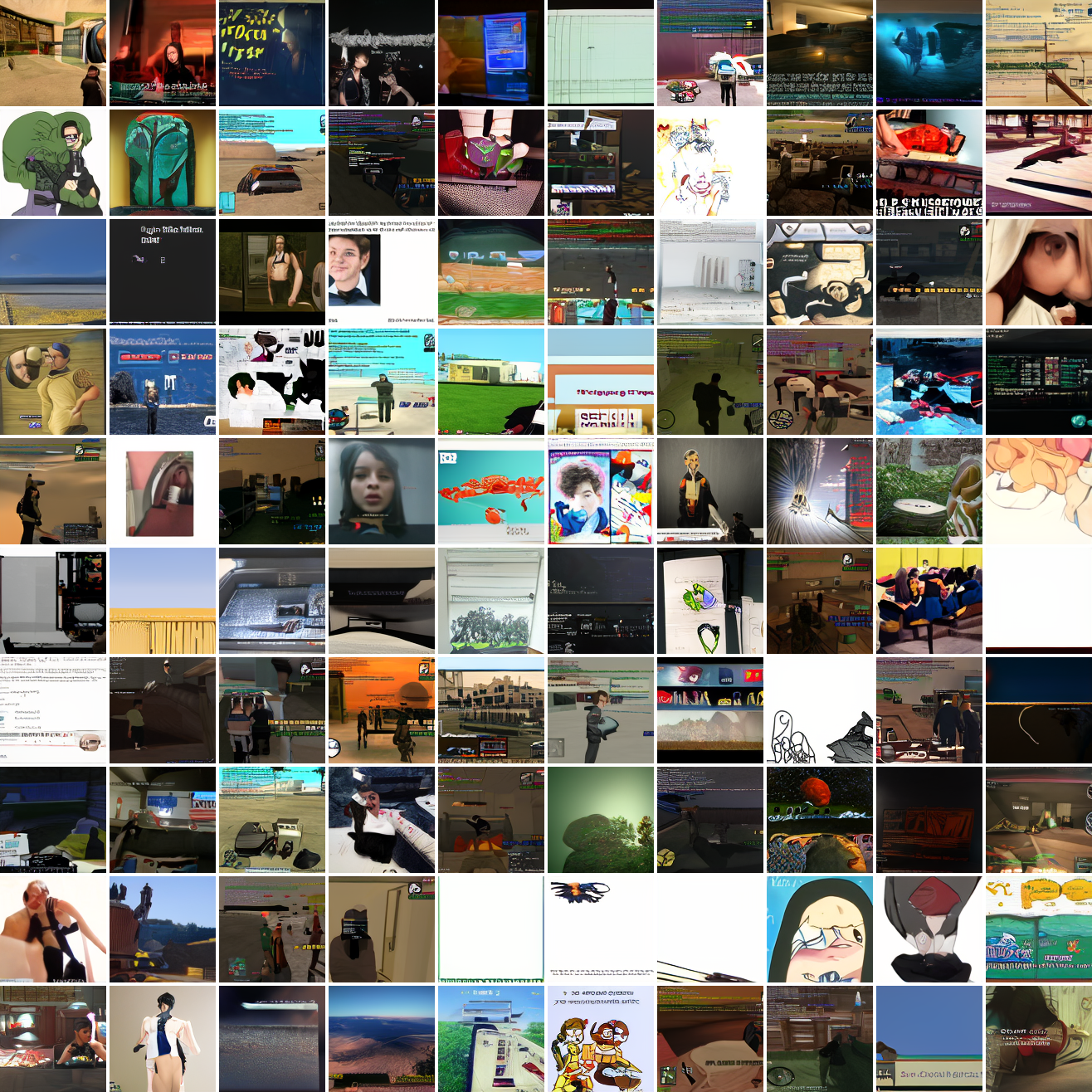
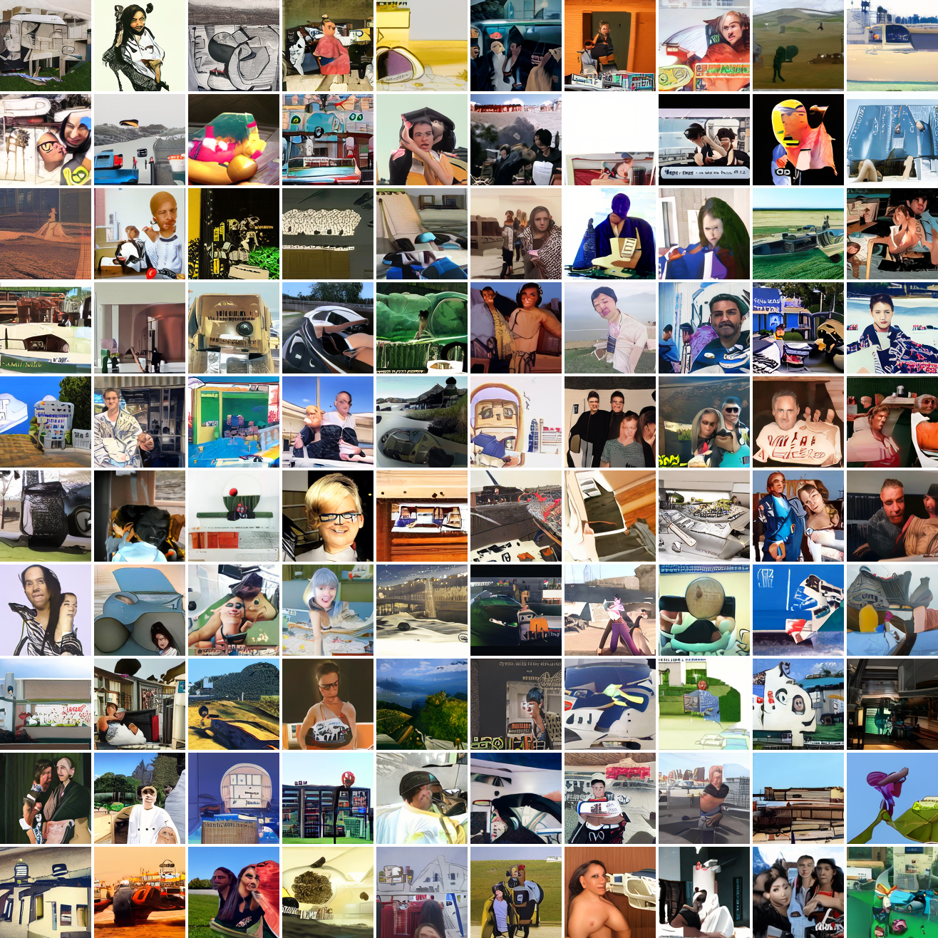
That’s the level of image quality you get from 25M images and 8 4090s for 82 hours2. Good enough for proof of concept, but not more. The two things my models are best at are faces and screenshots of GTA. Here are 100 samples conditioned on a GTA screenshot from the dataset.
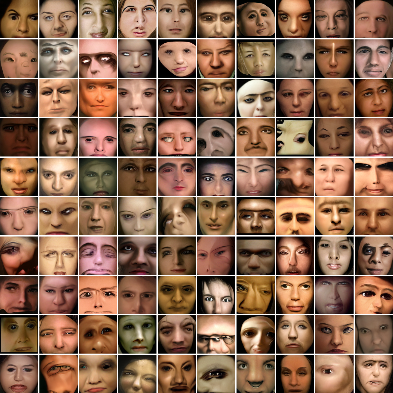
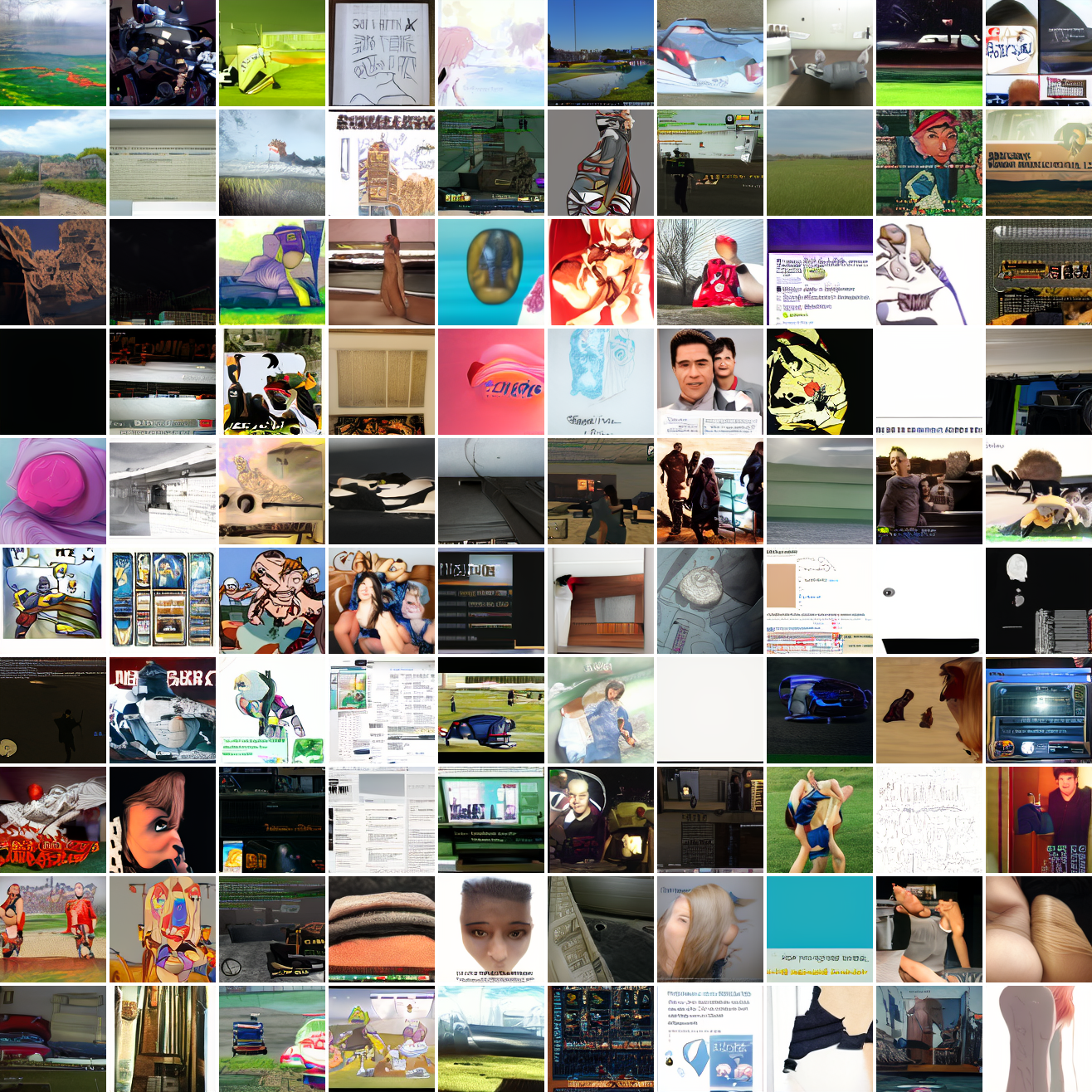
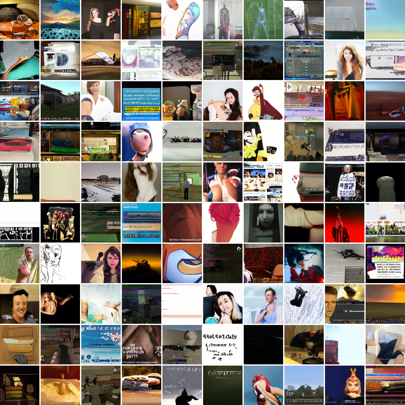
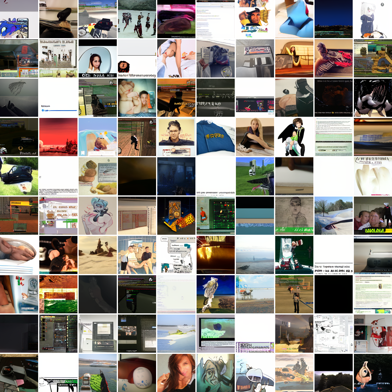
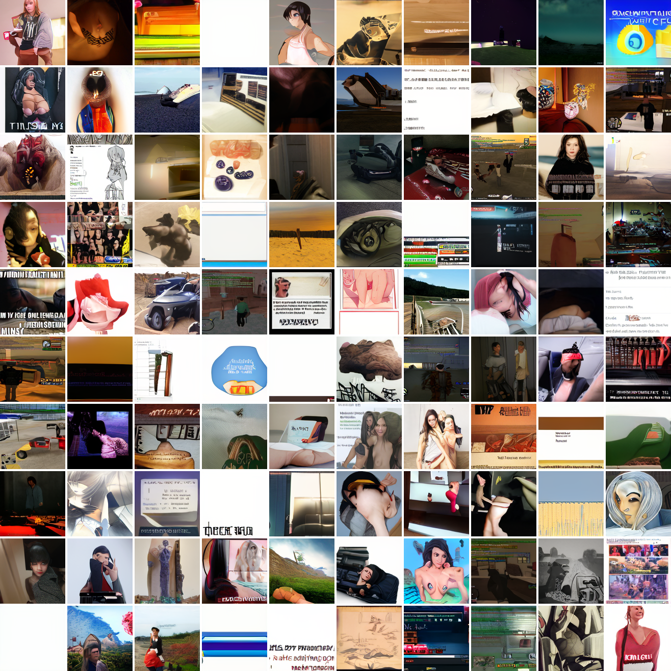
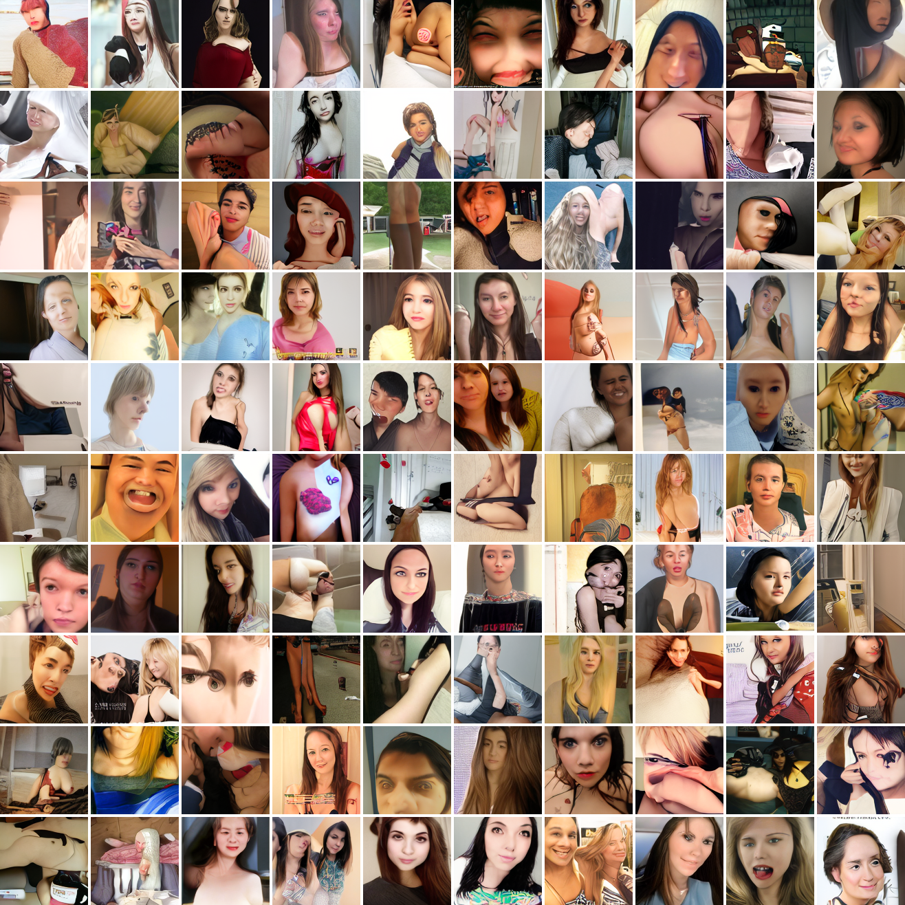
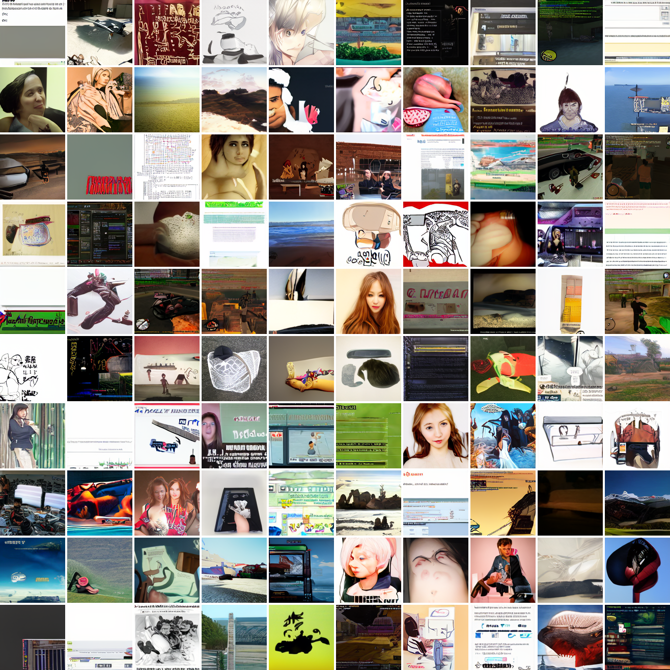
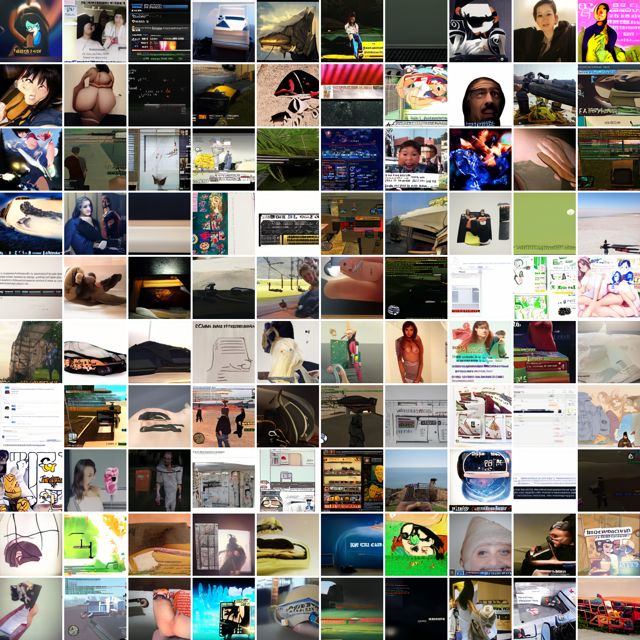
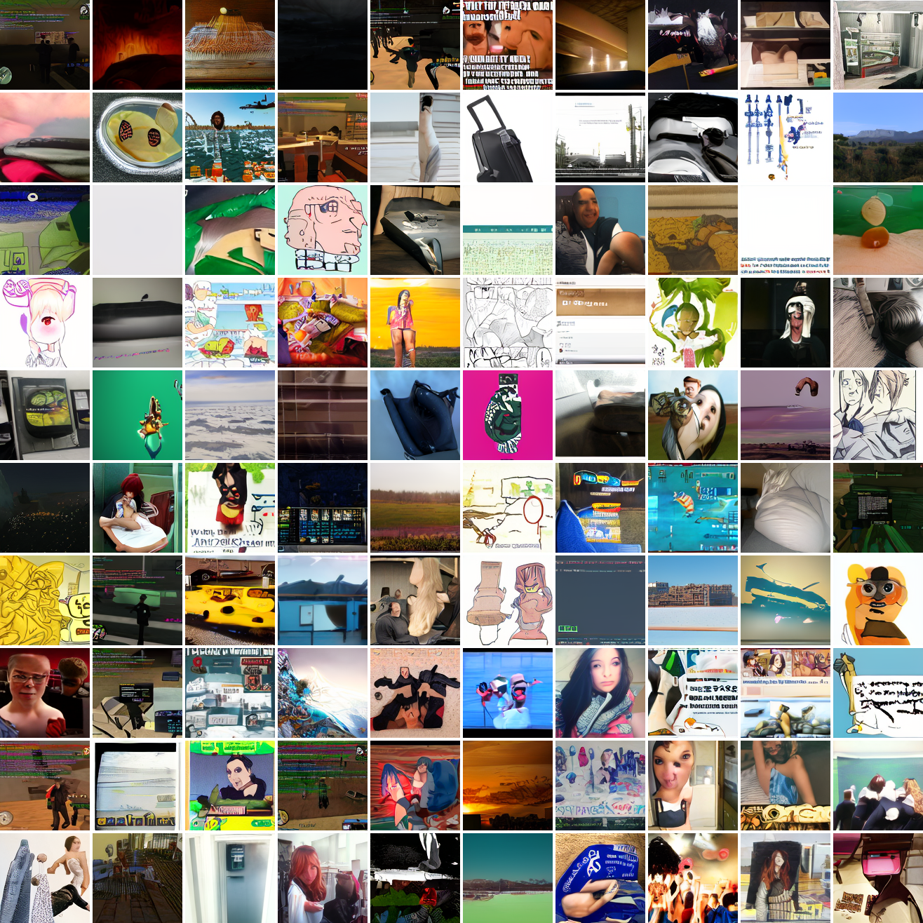
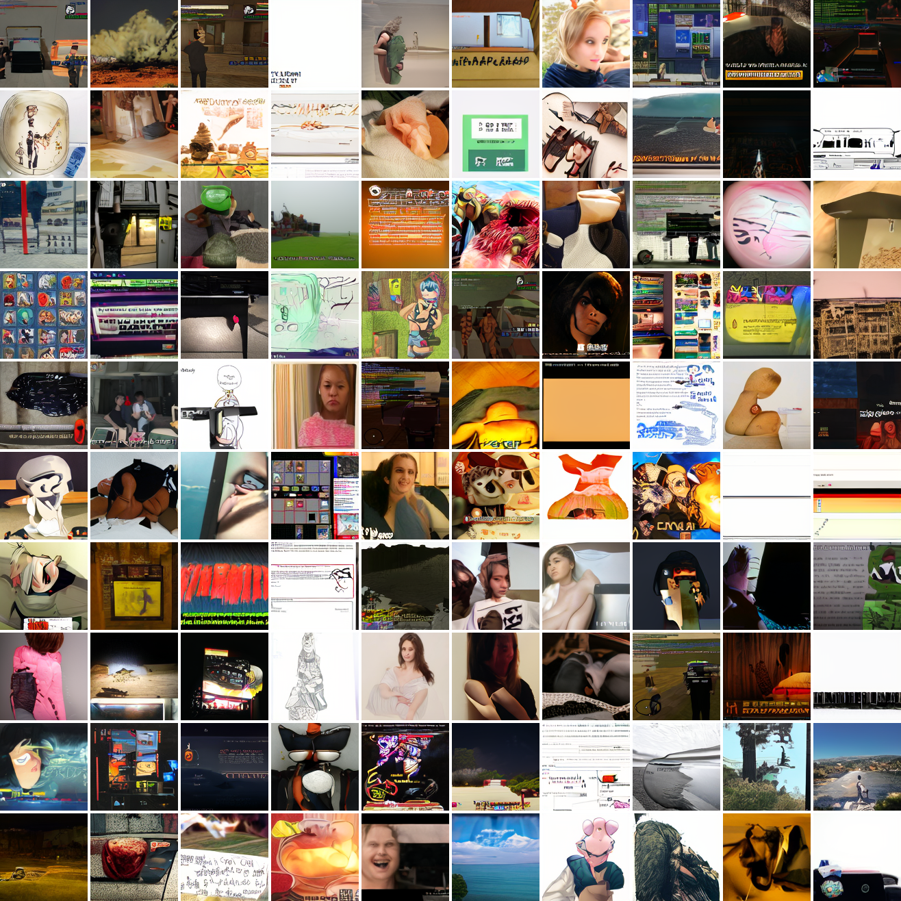
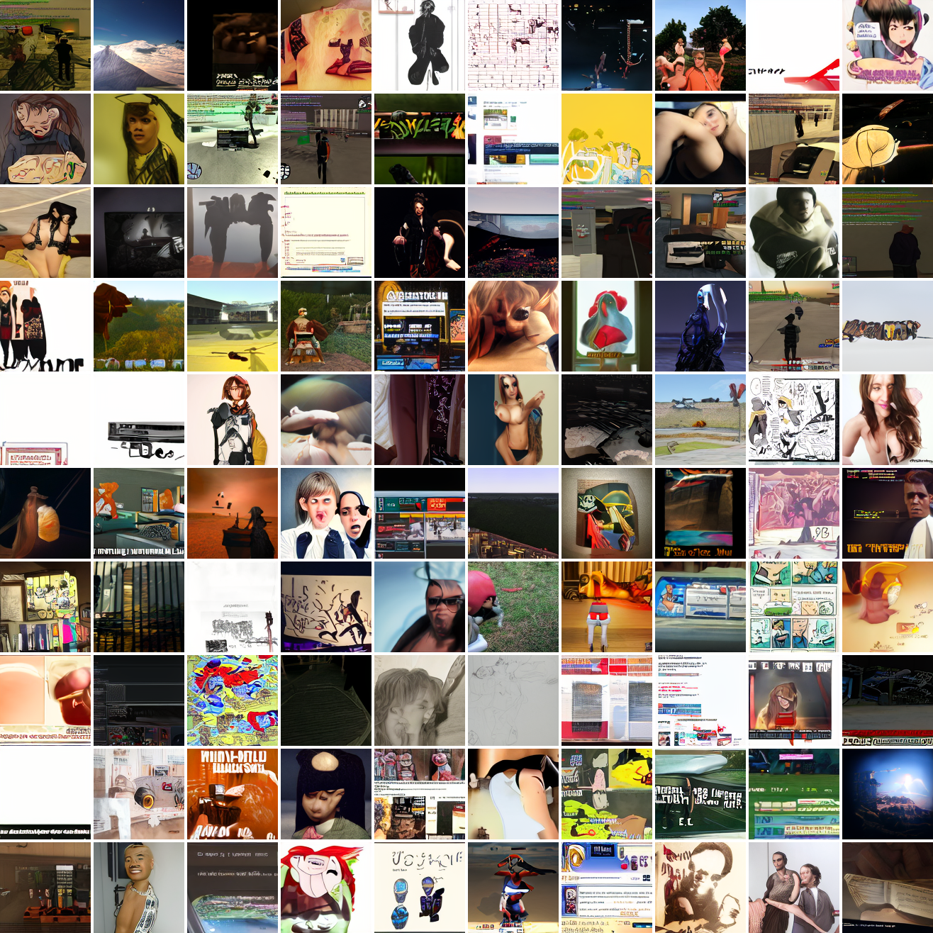
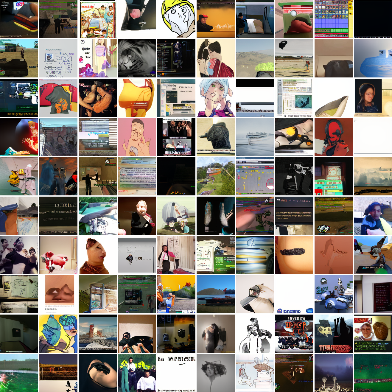
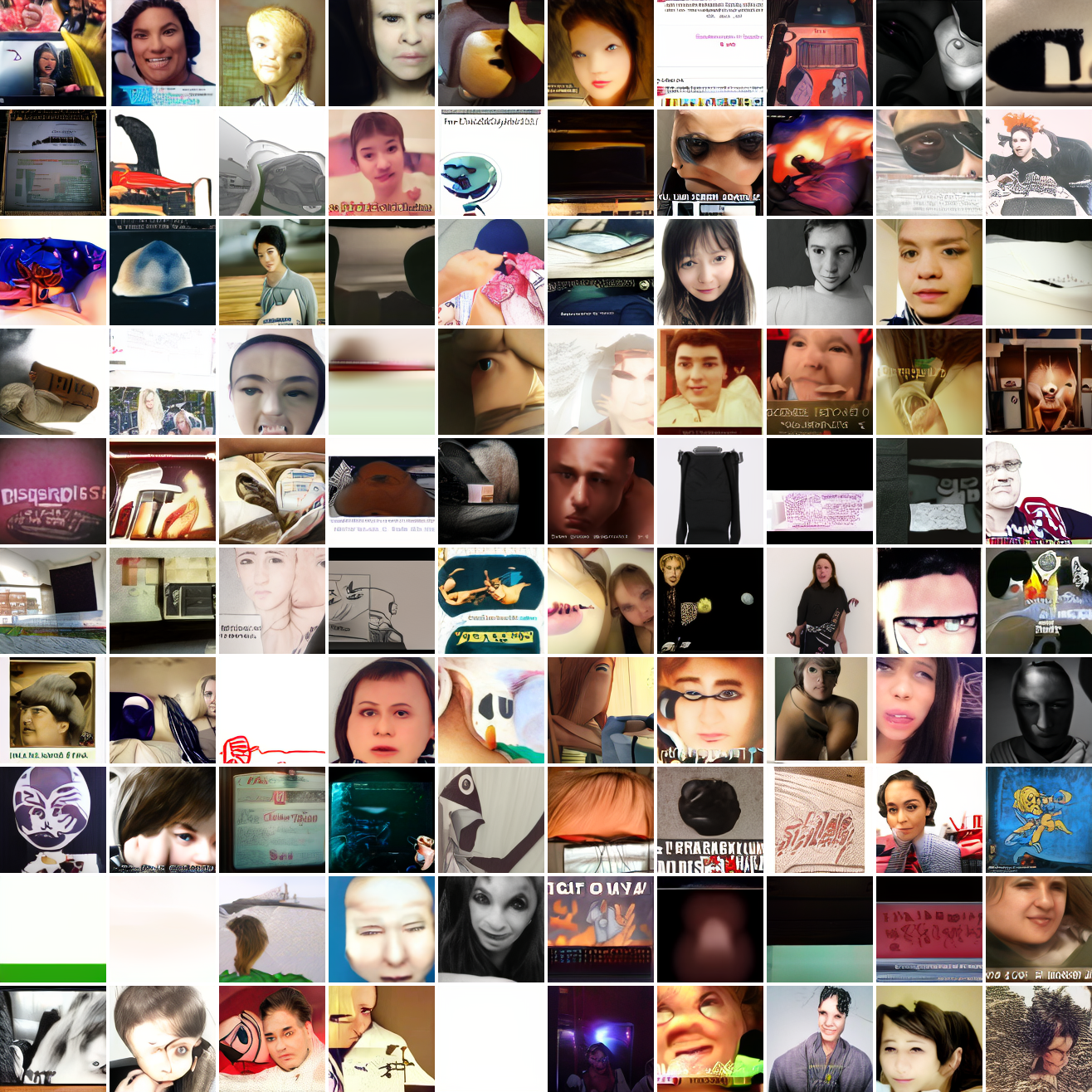
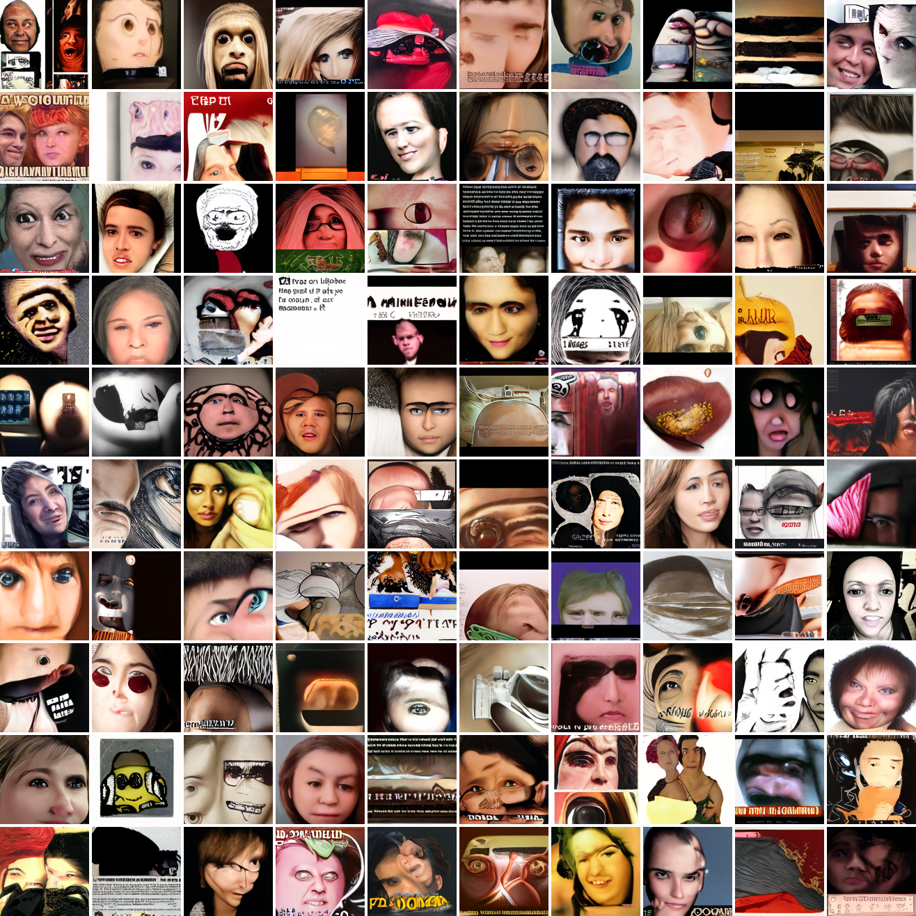
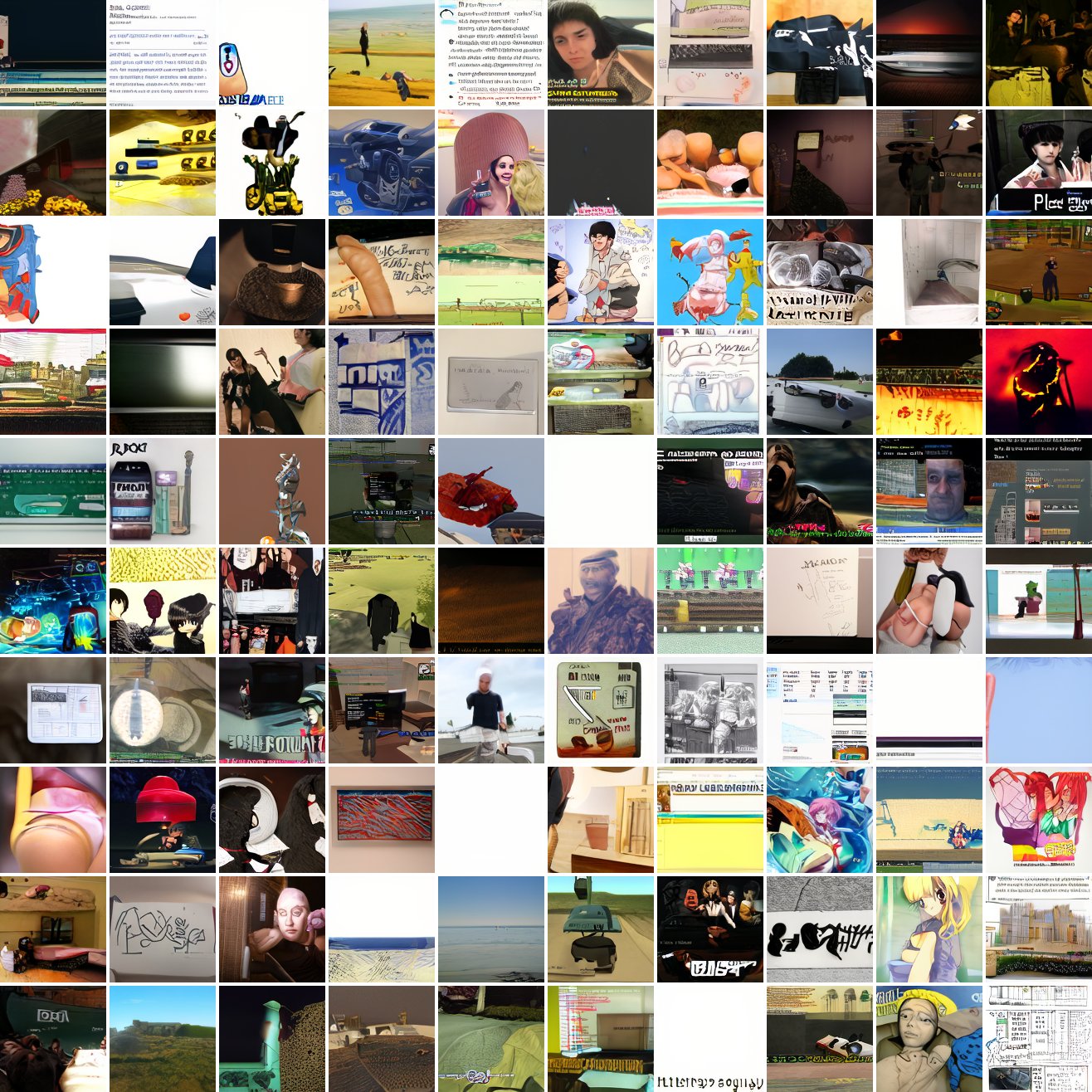
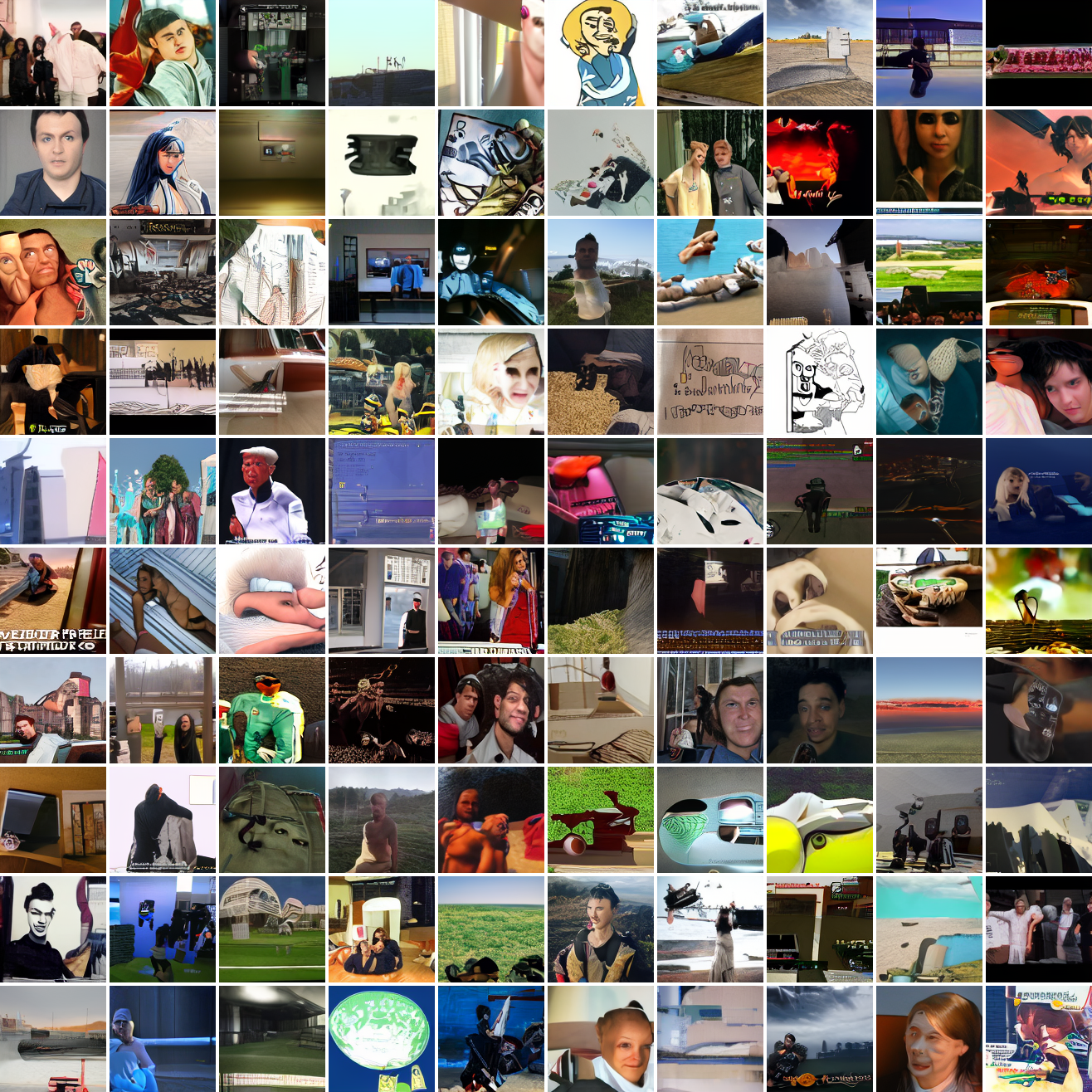
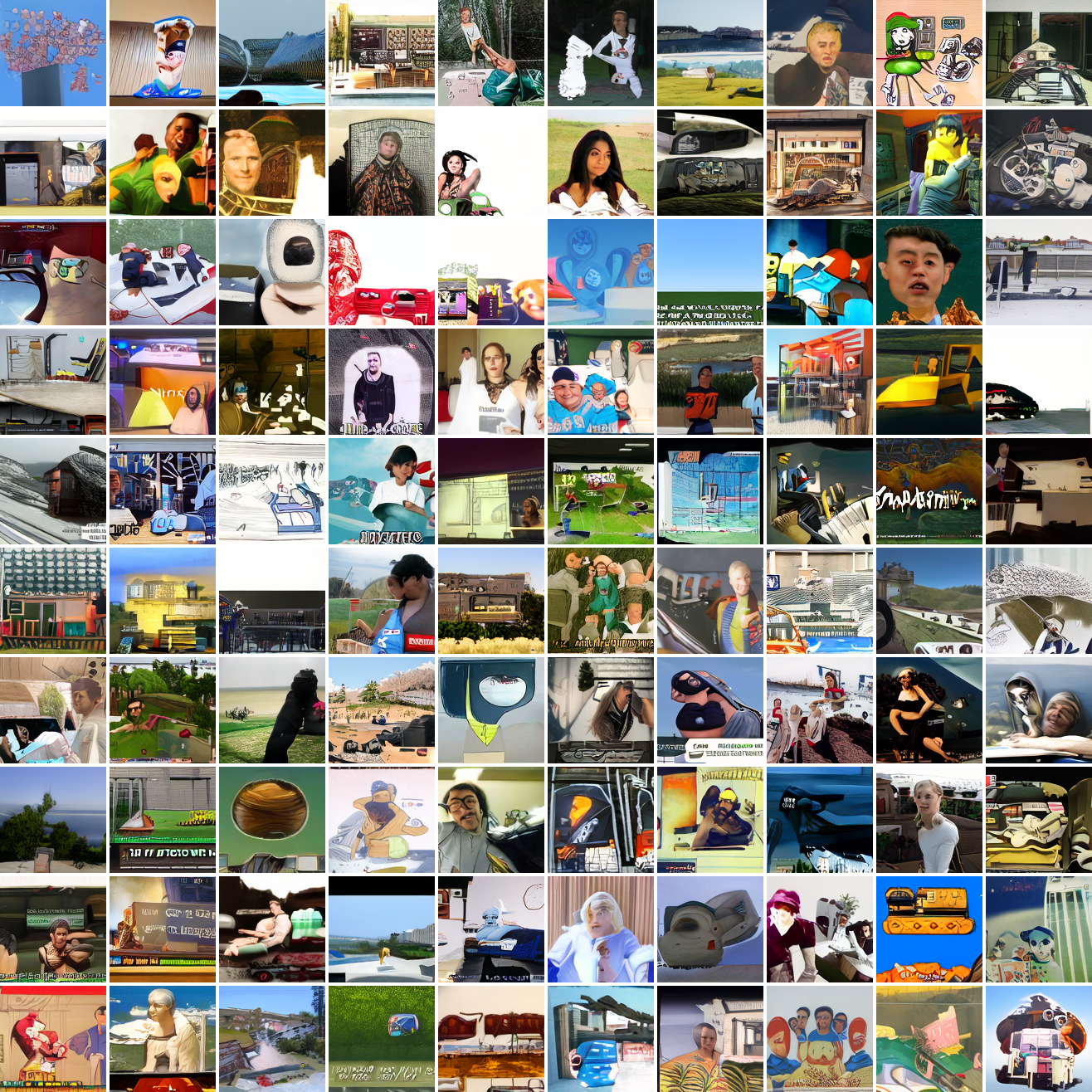
So, at least on image prompts, this baseline model works. Let’s try a couple matched text prompts. Here’s “A woman’s face”:
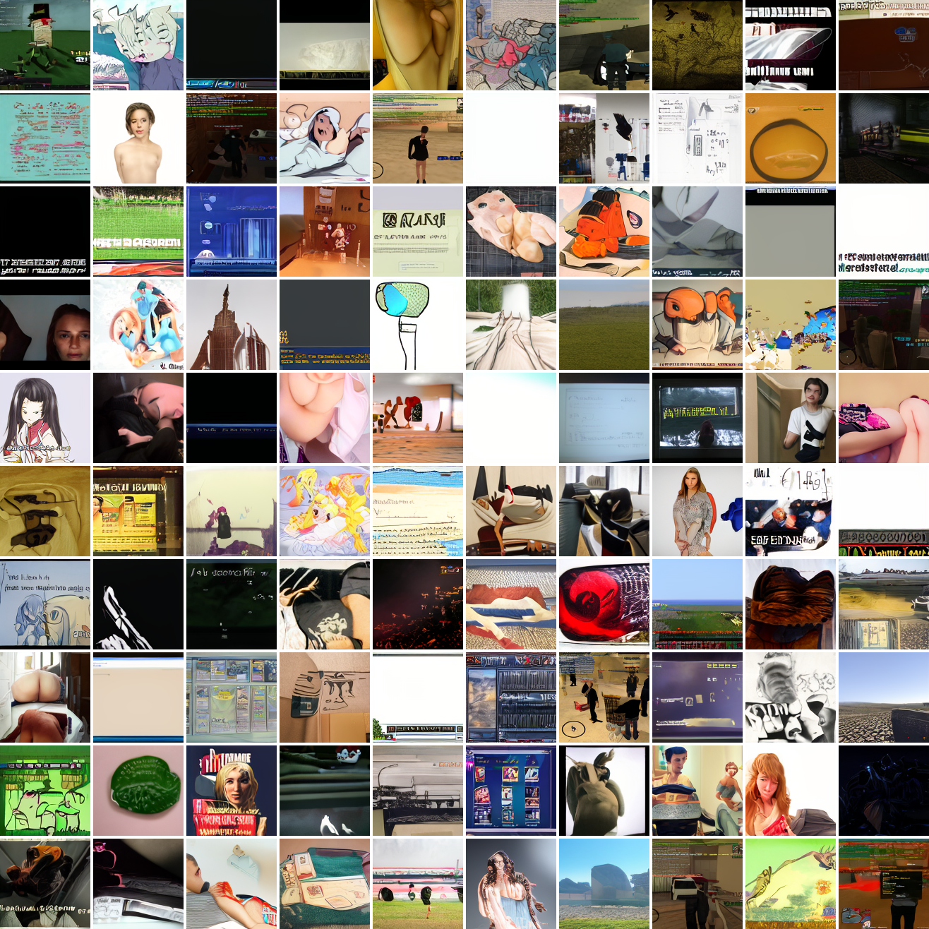
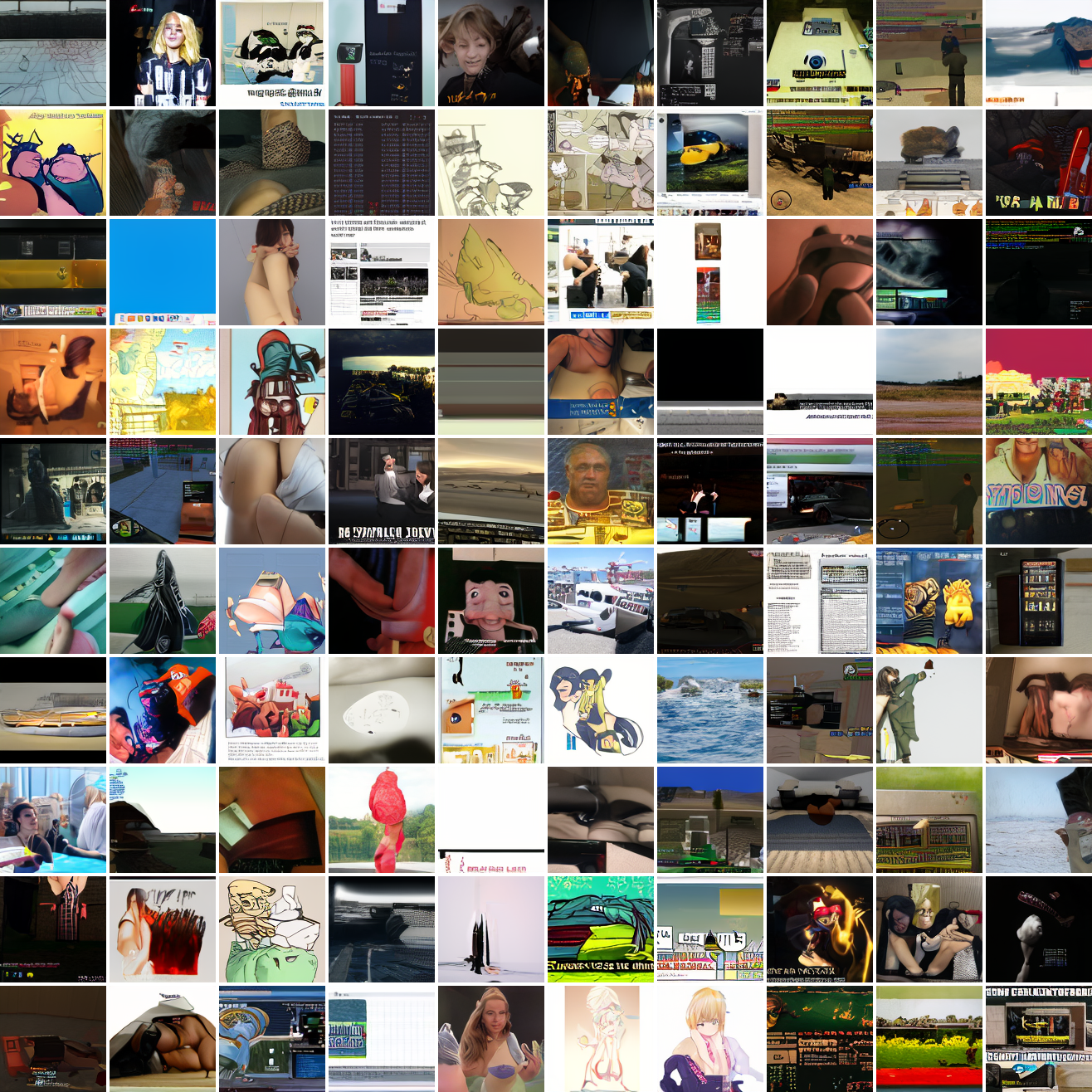
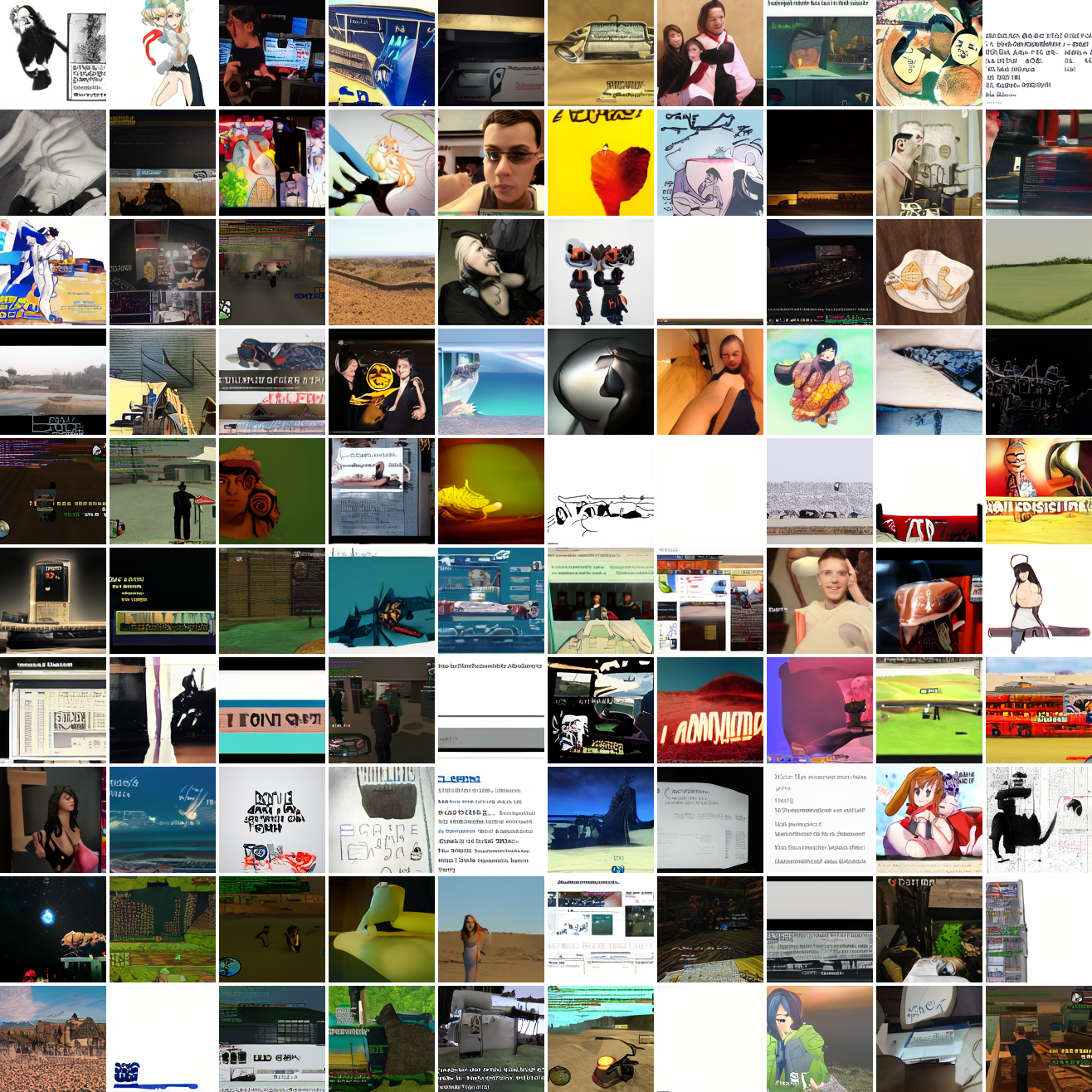
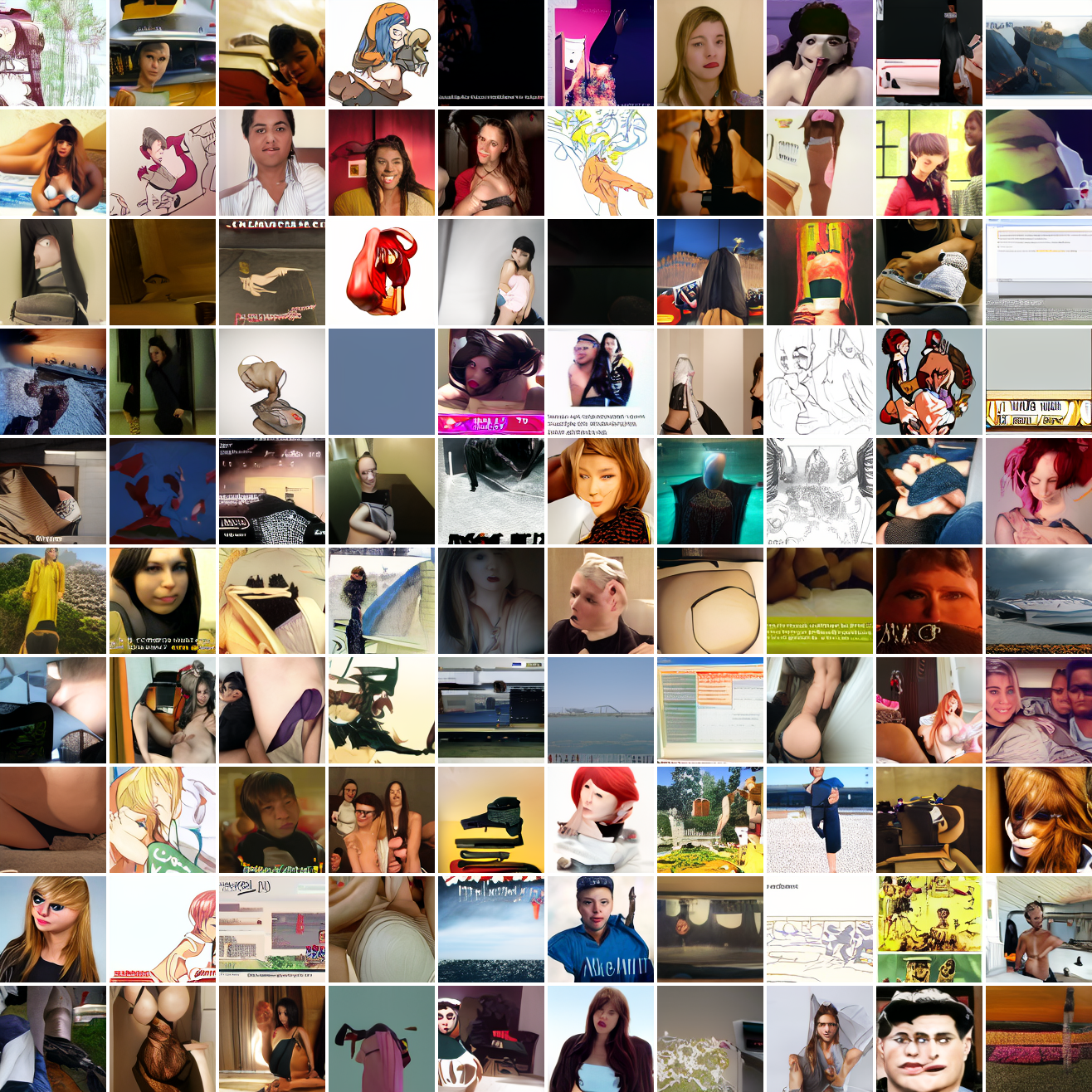
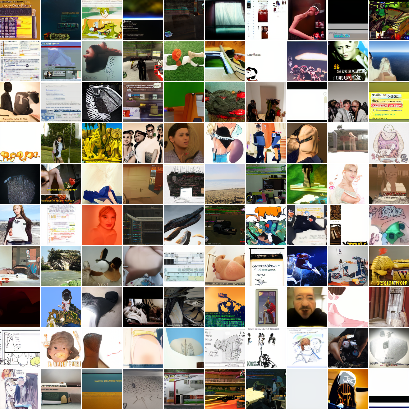
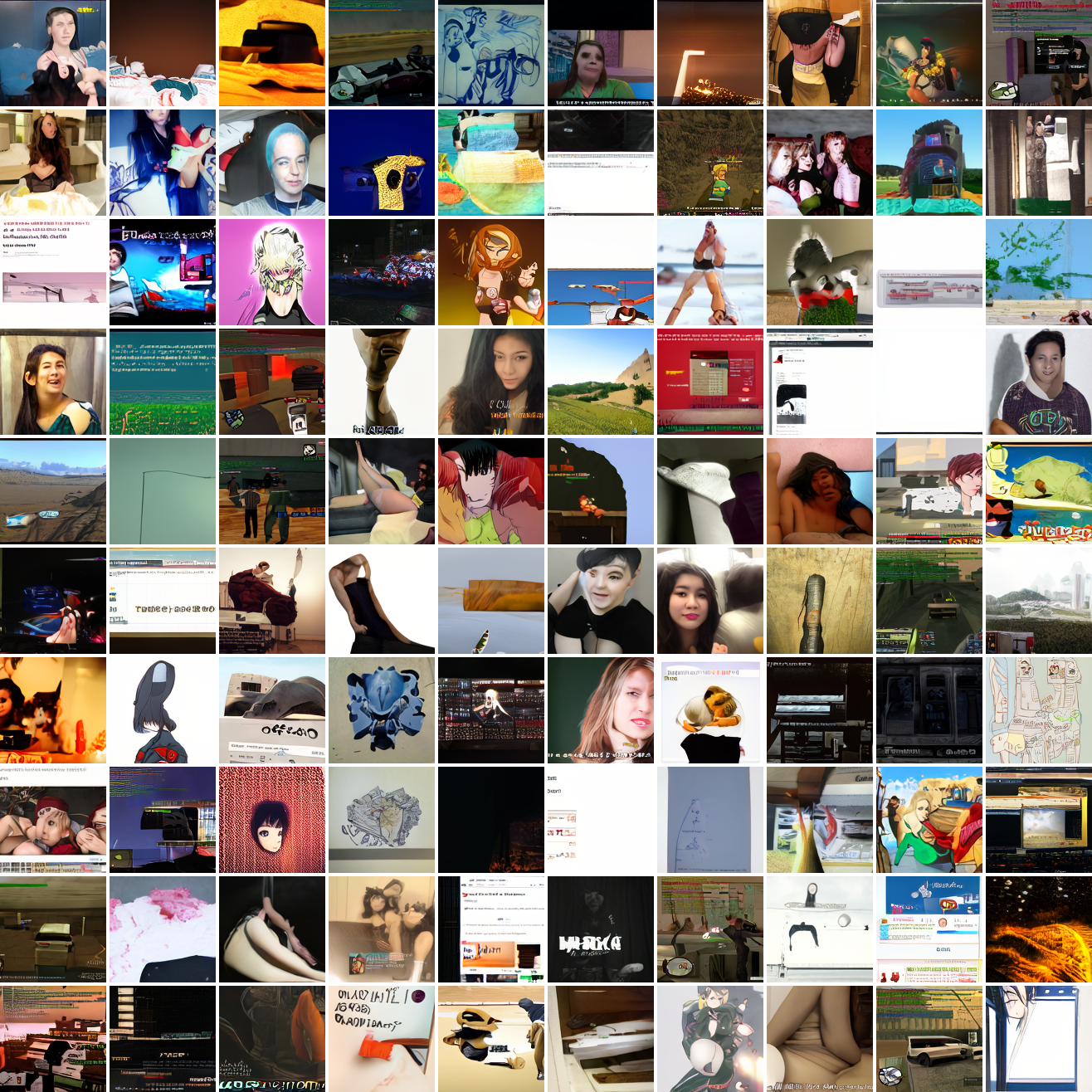
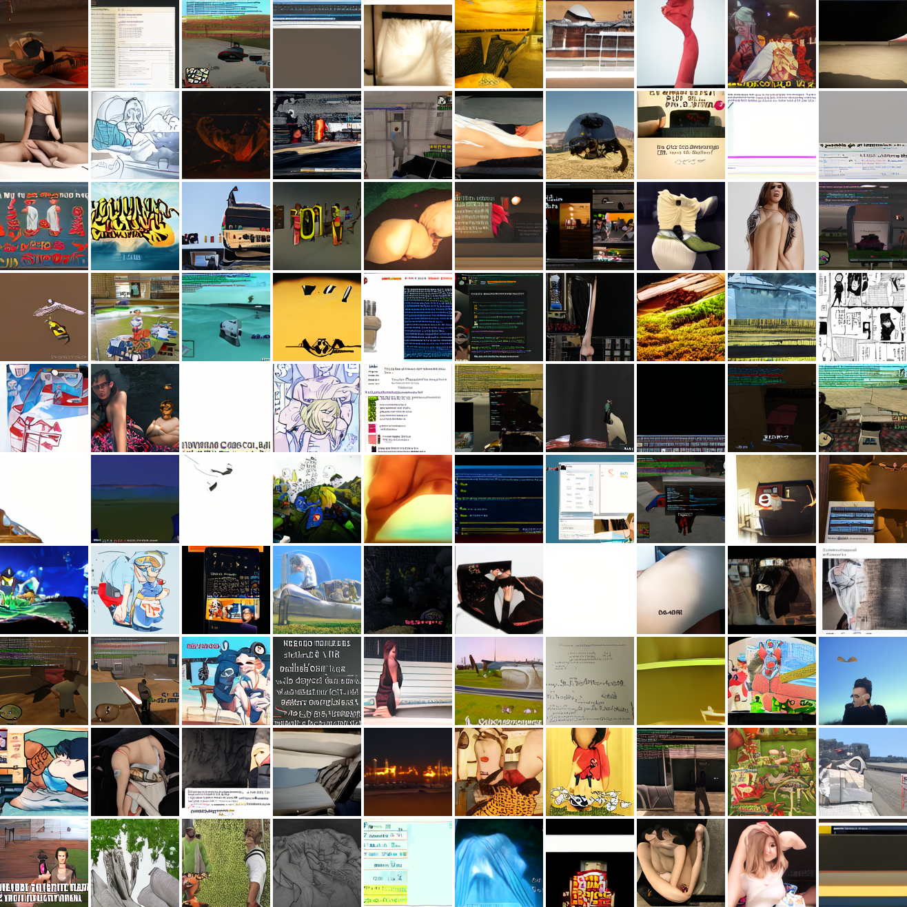
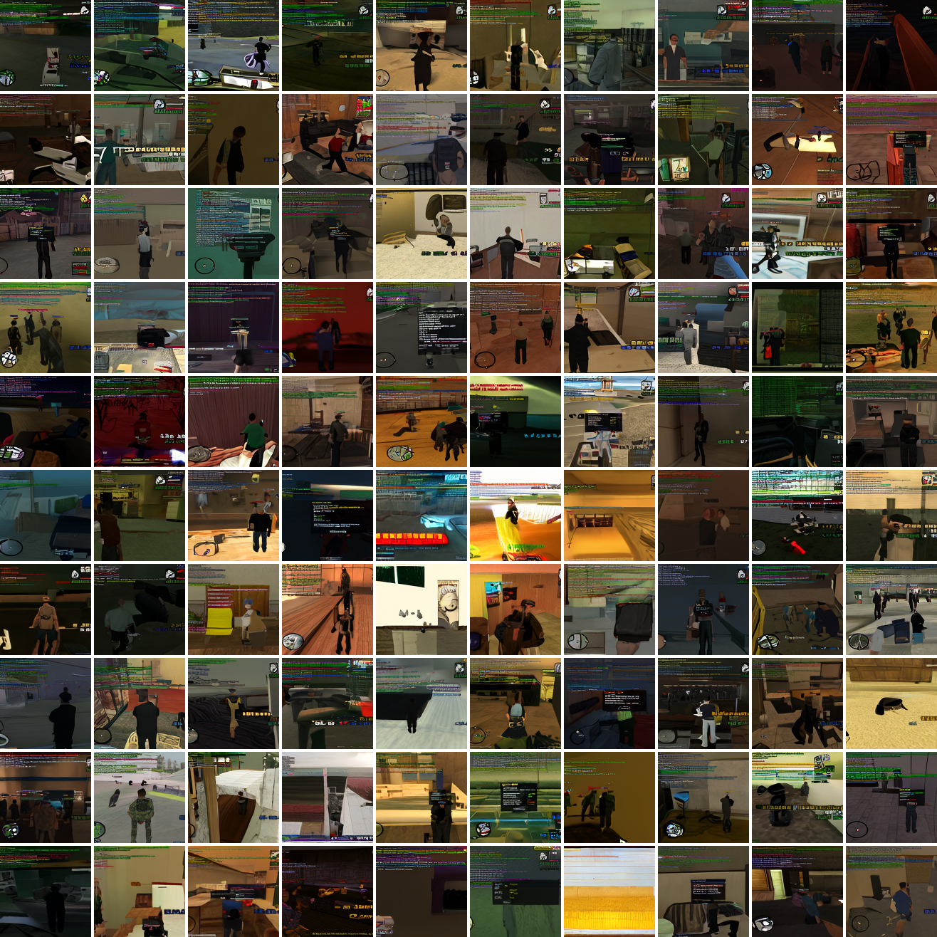
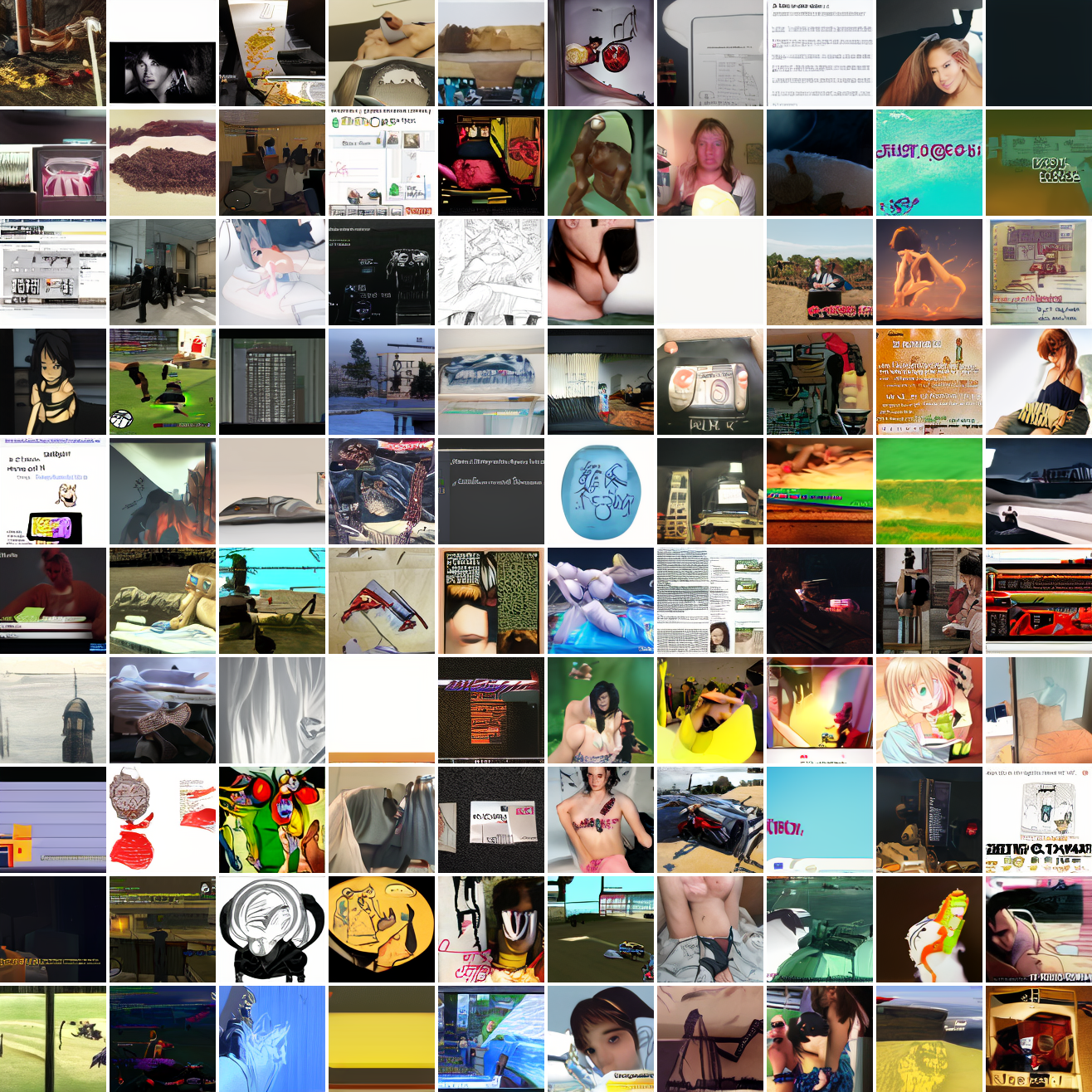
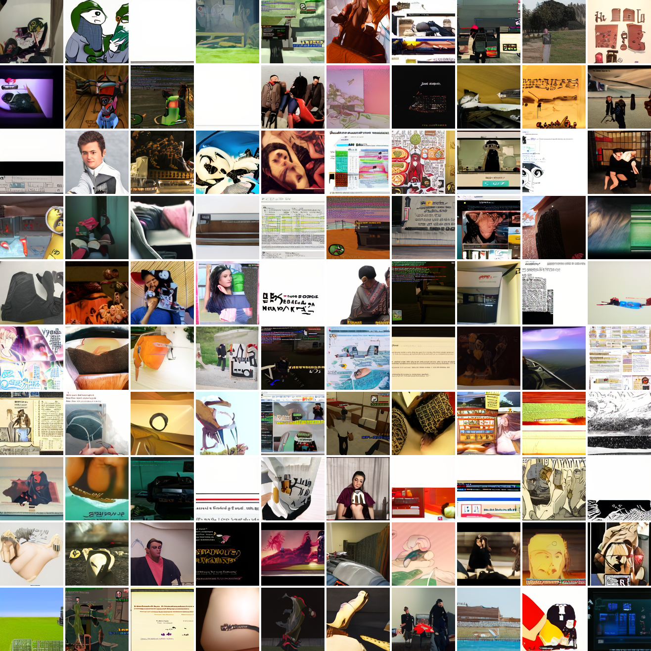
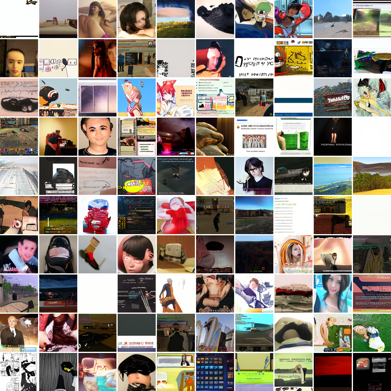
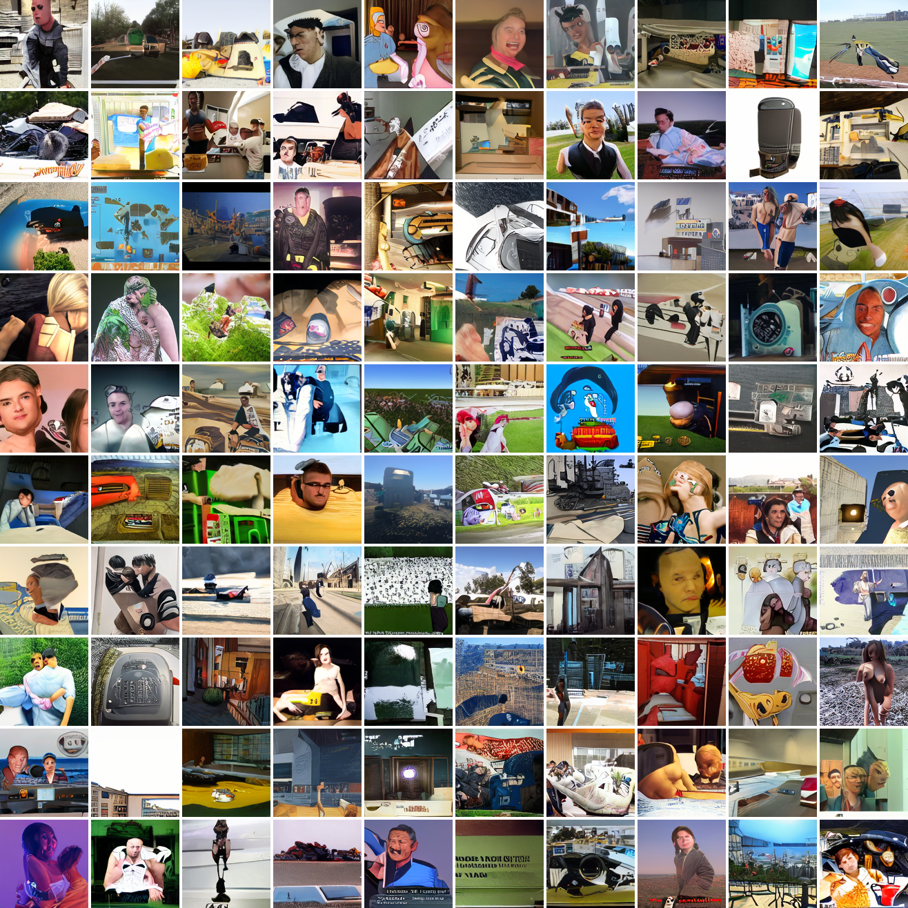
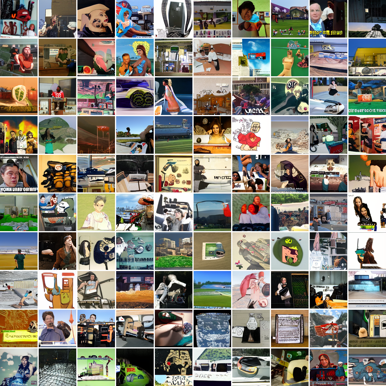
And here’s “A screenshot of Grand Theft Auto”:
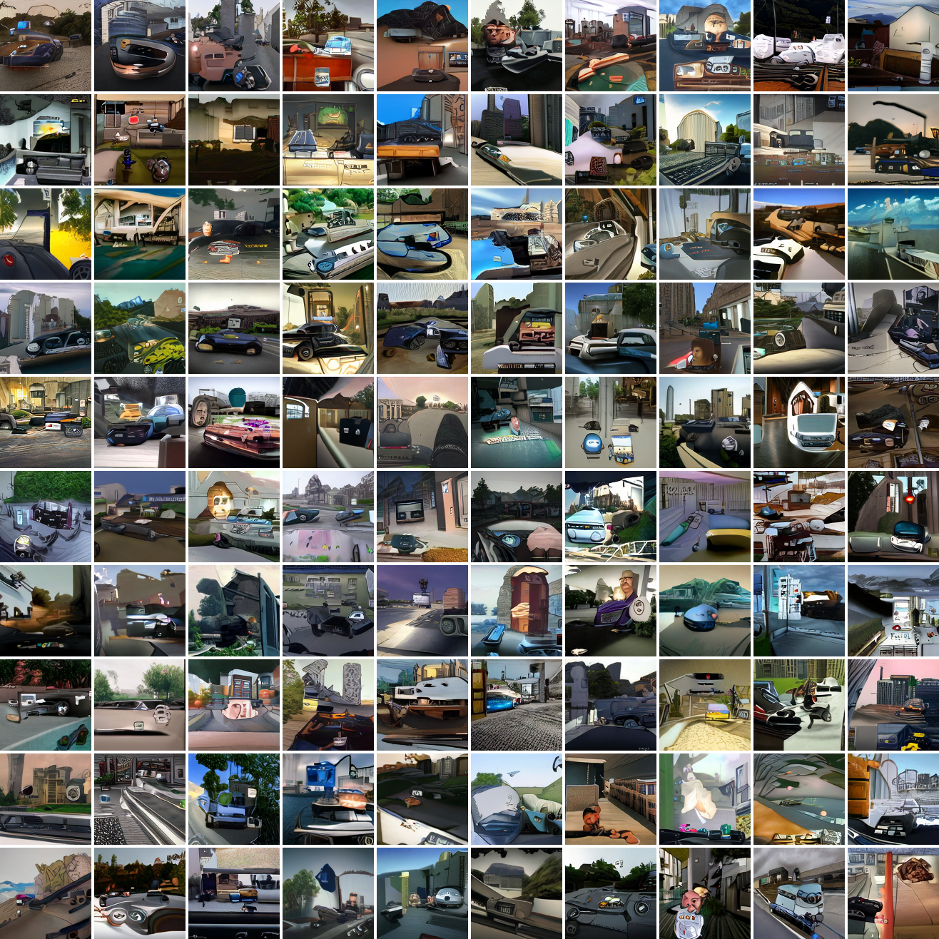
It generates faces, but they’re distorted, expressionless, posed weirdly, and sometimes off color. As for the GTA screenshot prompt, none of them look like GTA screenshots. They look like photos taken outdoors, and if we squint a bit we can see a lot of what might be cars. It’s much better at image prompts than it is at text prompts. Here’s the theory of why this should be the case:
The CLIP embeddings of images and captions are drawn from different distributions. CLIP’s objective puts images and reasonable captions for them close together, but that doesn’t mean they need to be on top of each other. An image’s embedding needs to be close to many possible captions’ embeddings simultaneously, and those caption embeddings need to be different so that they can be closer or further from different images. E.g. the photo of my friend’s embedding should be close to “a woman’s face”, “new haircut”, “day 2 at Burning Man”, etc. And since those emphasize different aspects of the photo, they should be separated. “A woman’s face” shouldn’t be closer to sideshaves than anything else, “day 2 at Burning Man” doesn’t necessarily need to be closer to images of people than images of sculptures, but does need to be near images that are in a dusty grey-orange place and far from forests or offices.
Furthermore, a model that learns to invert CLIP’s image projection function perfectly would generate images that had exactly the input CLIP embedding, which isn’t what you want. Instead you want images that are reasonably close to the input, for some definition of “reasonably close”.
Conditioning on a range
I went through several variations trying to get this to work. The first set worked at training time. The training code would choose either a range of distances or a concrete distance (depending on which version of the code we’re talking about), then sample a point with a cosine distance to the actual embedding within that range or with that distance from the real image embedding, and use that as conditioning data. This approach makes text embeddings in-distribution (provided the distances we choose cover the distance away captions tend to be), and the model should learn to generate ranges, but the distribution of images conditional on the range or distance is not what you want. Ideally the conditional distribution would be uniform over the possible images that have embeddings contained within the range, but a scheme that generates conditioning data based on the embeddings implicitly creates a distribution over the embeddings and not over the images. To make the distributions shaped like you want, you have to generate the conditioning data ahead of time and sample training images uniformly from the set that are inside the range.
Spherical caps in CLIP space
If we rephrase the “range” as a spherical cap, we can use the mathematical language that already exists to talk about them. (And talk to ChatGPT about them.) A spherical cap is a region of an (n-dimensional) sphere that is within some maximum angular distance from a vector. Since CLIP embeddings are unit vectors in 768-d space, we can define segments of CLIP space as caps. We have a central point in CLIP space and a maximum cosine distance, (defining the cap in terms of maximum angle or minimum cosine similarity is equivalent). Prompting the model with a cap centered on some point should generate images that are a maximum “semantic” distance from that point. So e.g. if you prompt the model with a cap centered on the embedding of the face above, a small maximum cosine distance should get you very similar images, and a larger maximum cosine distance should get you images that are still photos of faces, but not necessarily a similar looking person, a similar angle, light, etc. And a maximum cosine distance of 2 (covering the whole sphere) should be equivalent to unconditional sampling of the full distribution. A similar cap centered on the embedding of “The Golden Gate Bridge at sunset” should get you images that are pictures of the Golden Gate, but depending on the size of the cap, they might not be at sunset, or they might not be of that specific bridge. In addition, it’s important to note that the cosine distances between image embeddings and text embeddings don’t go below like 0.55. Even a very aligned image and caption are pretty far apart in CLIP space.
Sampling from the subset of a discrete set of unit vectors contained within a spherical cap
Since I’d decided I needed to generate caps and sample images from the training set that have embeddings within them, I needed to write software to do this. It was exceedingly difficult to do this efficiently. My run generating 25M cap-image pairs took around 4 days. And that’s after a lot of optimization effort. It runs at like 20-25% GPU utilization. So there’s a lot of room for improvement (I sure as hell hope so anyway). One should not write high performance code that needs to do a lot of work on the CPU as well as the GPU in Python. Or using JAX, probably. If I ever get around to doing a rewrite it’ll be in Rust and deal with the GPU at a lower level. Anyway, notes on what I did do:
A space partitioning data structure for unit vectors
I organize the vectors into a tree of spherical caps. Each tree contains a set of vectors, a central vector, and a maximum cosine distance. Every vector has a cosine distance to the central vector less than or equal to the maximum cosine distance. Leaves directly contain vectors, and nodes contain a set of k children, where k is a configurable integer constant >= 2 (in practice 64 or 128). Initially, the tree consists of a single leaf which has an arbitrary center and a maximum cosine distance of 2 (the opposite side of the sphere). Then, leaves are split recursively until all leaves are smaller than some configurable maximum number of vectors.
To split a leaf into a node and a set of children, I do k-means on the vectors in the leaf. The centroids become the children’s central vectors, and the maximum cosine distances are computed by iterating over the vectors in the children. Leaves are split until they contain less than some configurable maximum number of vectors.
I call this structure a captree. This structure has two important properties for sampling. First, you can test whether two caps intersect, and whether one contains the other, based only on the cap geometry. When sampling vectors in a captree that are contained within a query cap, you can eliminate any subtrees from consideration whose caps don’t intersect the query cap; if the query cap contains the entire cap of a subtree, then you can skip looking inside that subtree. Second, clustering the vectors at the top level means matching vectors are more likely in some subtrees than others, which makes approximate sampling work better.
Aside: Infinidata
The CLIP embeddings of my 25M image dataset are ~72GiB. That doesn’t fit in RAM on my home machine, though it does fit on bigger servers. I wrote a library for manipulating big datasets that don’t fit in RAM called Infinidata. Initially, I tried to use Huggingface’s Datasets library, but it was way too slow and ate tons of RAM and disk space. In general, Datasets is fine if you’re just downloading stuff, shuffling stuff, loading stuff or iterating over it in batches, but there’s all this other functionality and I get the vibe that nobody seriously uses it. Infinidata allows me to do the leaf splitting operation without copying while keeping the vectors out of RAM.
Two stage sampling
Sampling proceeds in two phases, an approximate algorithm that works on ~80% of queries and an exact algorithm that works on the remainder, is much slower, and takes the majority of the overall runtime.
The approximate sampling algorithm operates non-recursively at the top node and proceeds by estimating the number of vectors in each immediate child subtree that are contained within the query cap. First it computes the intersection status of each child’s cap with the query cap. Children that are fully contained by the query naturally have all of their vectors match, and children that don’t intersect have zero matches. For children that intersect the query cap but are not contained by it, we estimate the number of matching vectors by sampling uniformly inside that child. Our estimate is the fraction of samples that match times the number of vectors in the child. Once estimates have been computed for all children, we sample from the children in proportion to their estimates. For the fully contained children we sample from all their vectors, and for the intersecting children we sample from the matching vectors that we sampled from to estimate the number of matches. The number of samples used for density estimation is a tradeoff between sampling time, bias, and, when doing batched sampling, duplicate rate.
If the approximate sampling algorithm finds zero matches, sampling falls back to an exact algorithm. If we were willing to accept false negatives we could skip it, but it’s important in this application for the training examples to include small caps that contain few or one vectors. Exact sampling works by enumerating the matches in every subtree and sampling from them. This is conceptually straightforward. A lot of engineering effort went into making the vector checks asynchronous, batching, and various microoptimzations. Python is not a fast language, and dumb stuff like accessing a foo.length property directly instead of calling len(foo) can make a big difference.
Batched sampling
A lot of the costs of sampling can be amortized across multiple queries. In approximate sampling you can share the density estimation samples across queries, and in exact sampling the work of loading the vectors in leaves and shipping them to the GPU can be shared. This stuff makes a huge difference and is necessary to make sampling performance at all tolerable.
Generating the caps to sample from
CLIP space is large and high dimensional, and we want some of our caps to be very small. This means that generating caps with uniformly distributed centers is untenable - the vast majority of the small caps will be empty, meaning the generated training examples would disproportionately have large sizes. My approach is this is simple: to generate a cap I sample two vectors from the set of embeddings we’re generating from, generate a value in U[0, 1], and do spherical linear interpolation between the two vectors, using the value as the interpolation parameter. To get more useful conditioning data, I draw the maximum cosine distances non-uniformly. 95% of the time they’re drawn from U[0, 1], the remaining 5% of the time they’re drawn from U[1, 2]. Since users are mostly going to use the model with distances below 1, and since smaller caps provide more information at training time, this seems like a good idea. Given the results discussed below it’s hard to tell whether this achieves the goals, but it’s simple and seems logically sound.
Cap conditioned results
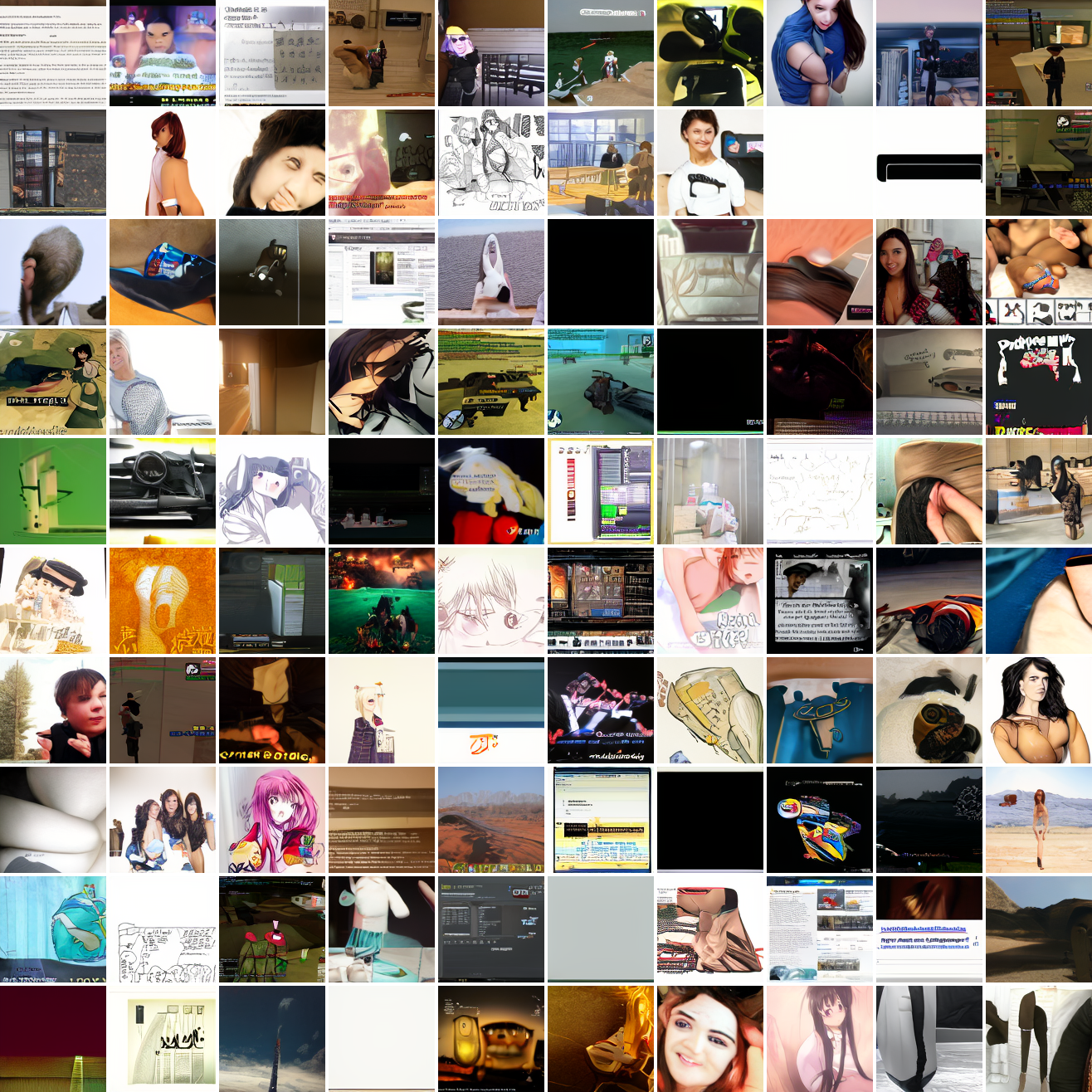
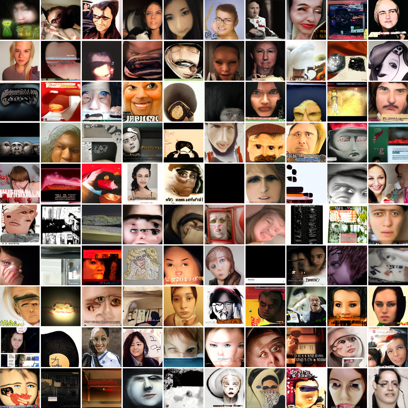
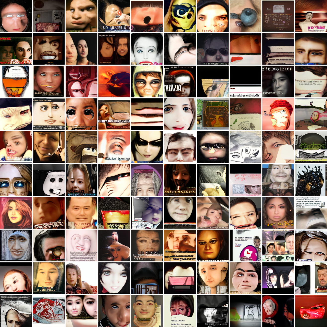
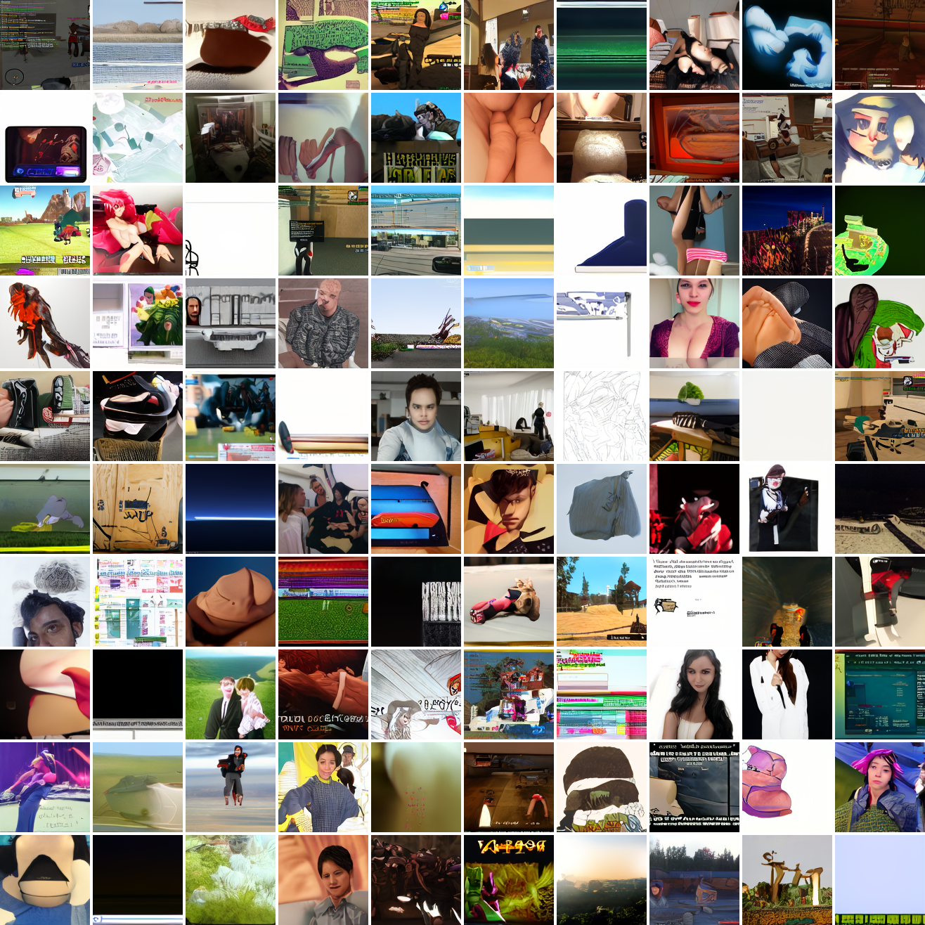
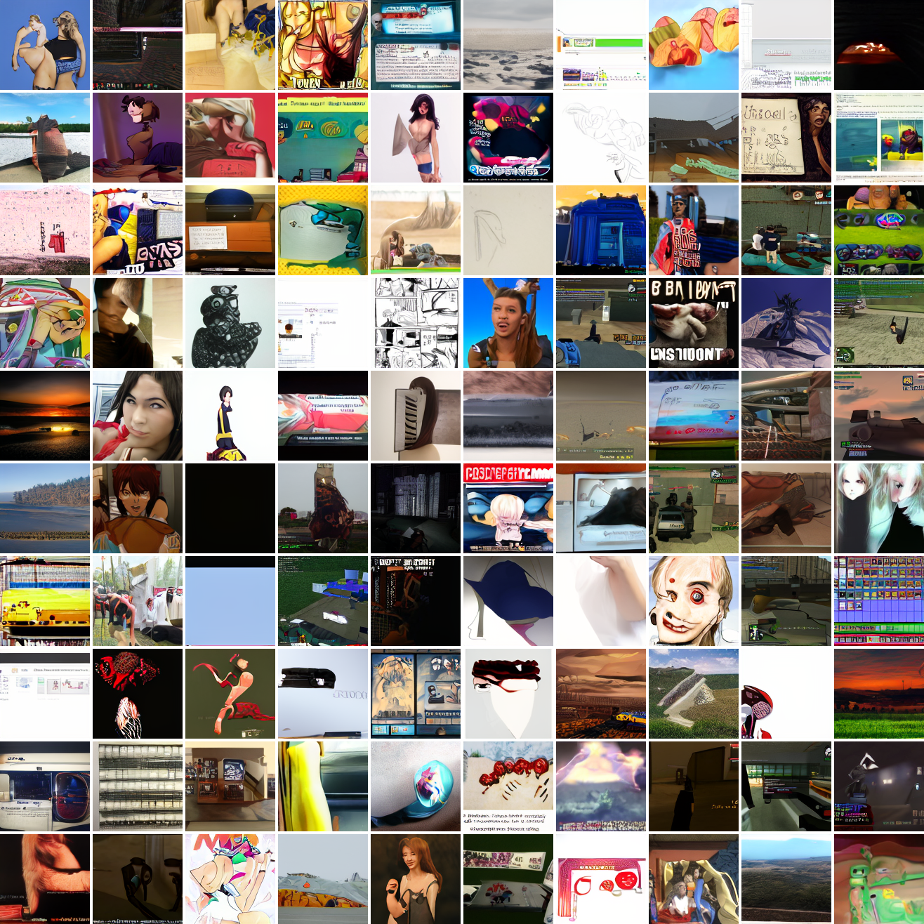
My cap conditioned model achieves losses very close to the baseline model, but the samples are not as good as one would hope. Here’s a series of images conditioned on the embedding of the same photo of my friend, with max cosine distances from 2.0 (the entirety of CLIP space) to 0.0 (a point). Note that the surface areas of these caps is nonlineary related to the max cosine distance. The surface area is heavily concentrated near the middle when working in high dimensions - while the cap with max distance 2.0 covers the entire sphere and the cap with max distance 1.0 covers half the sphere, the cap with max distance 0.5 covers way less than a quarter of the sphere.
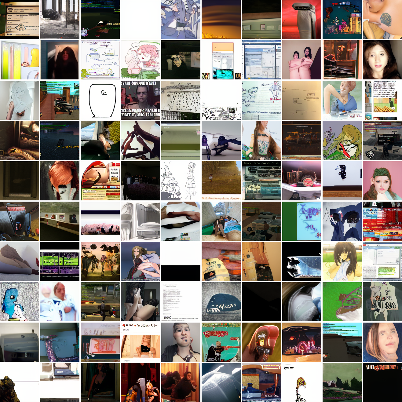
At max cosine distance 2.0, the samples are highly diverse and largely incoherent. Of the images where you can actually tell what it is, there are screenshots of websites, faces and figures, screenshots of video games, screenshots of GTA, and landscapes. This pattern continues up until around 0.5, when faces become the most common type of image. As the size of the cap continues to get smaller, the images get more consistent, with the pose and positioning of the faces becoming more homogenous.
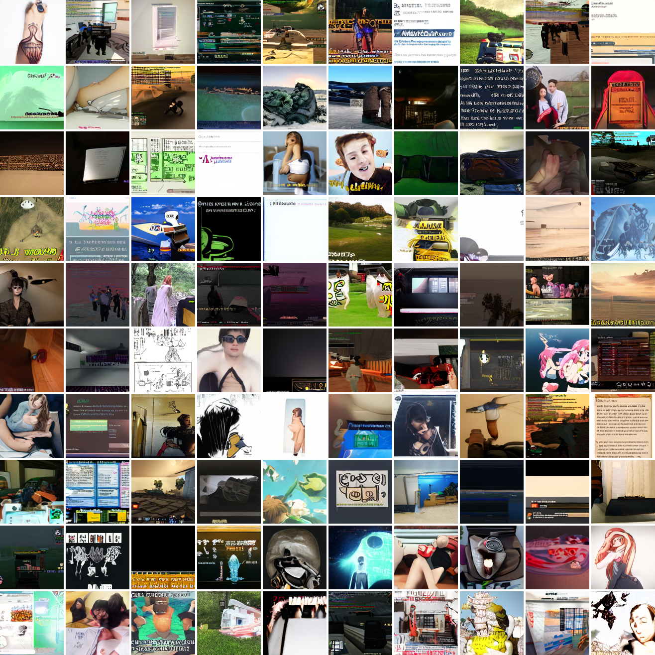
Now let’s see a similar series of images conditioned on the embedding of a GTA screenshot.
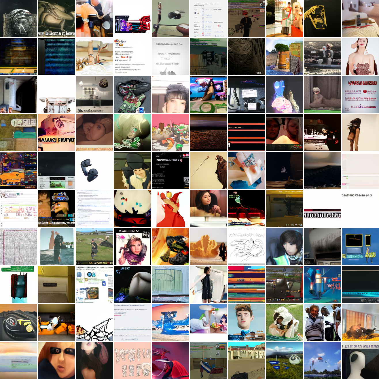
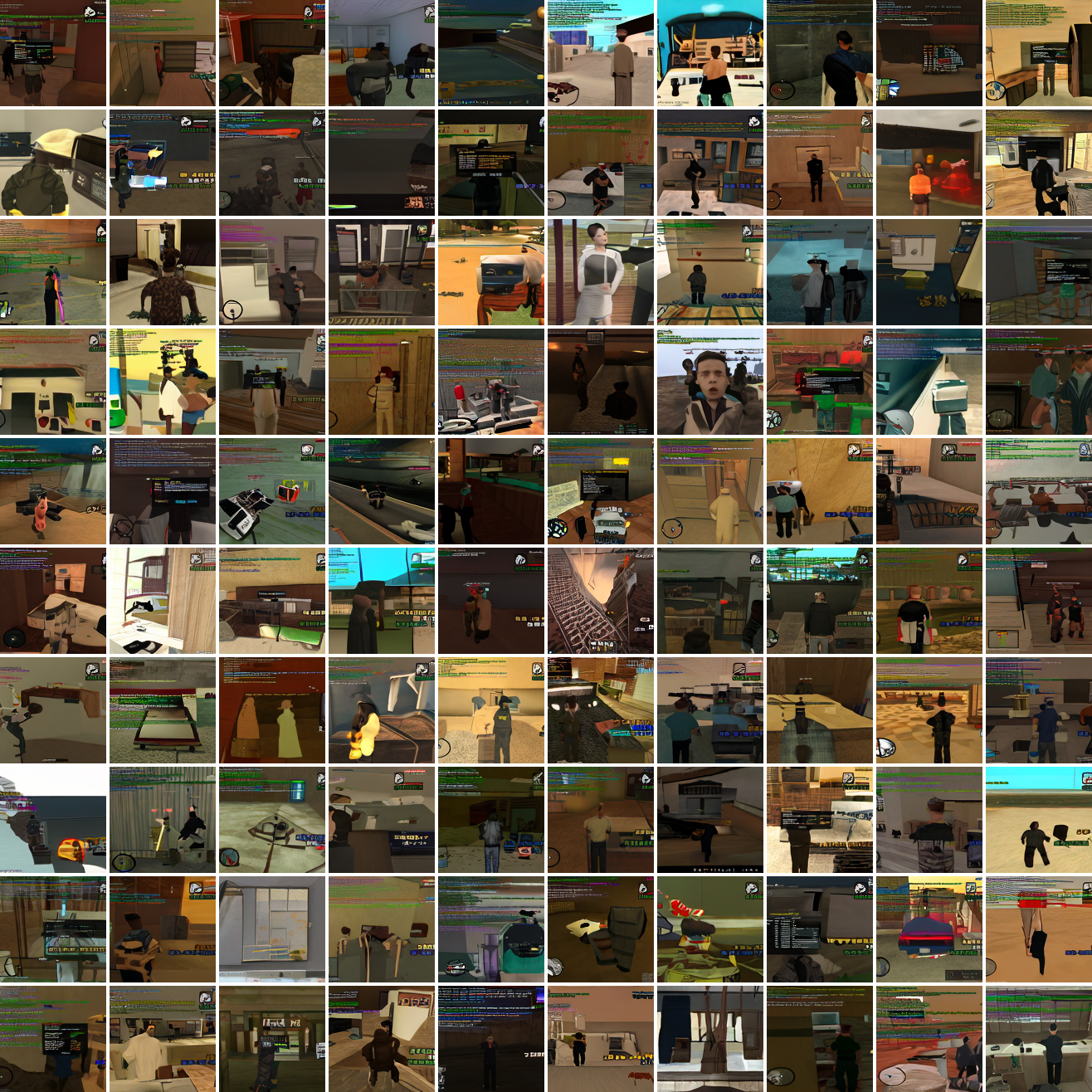
This is about what you’d expect from a model like this, but in a good model you’d start seeing mostly faces or mostly screenshot type things around 0.9 or 0.8.
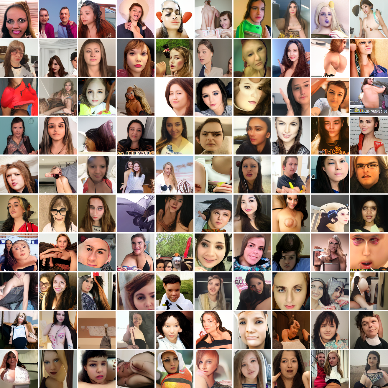
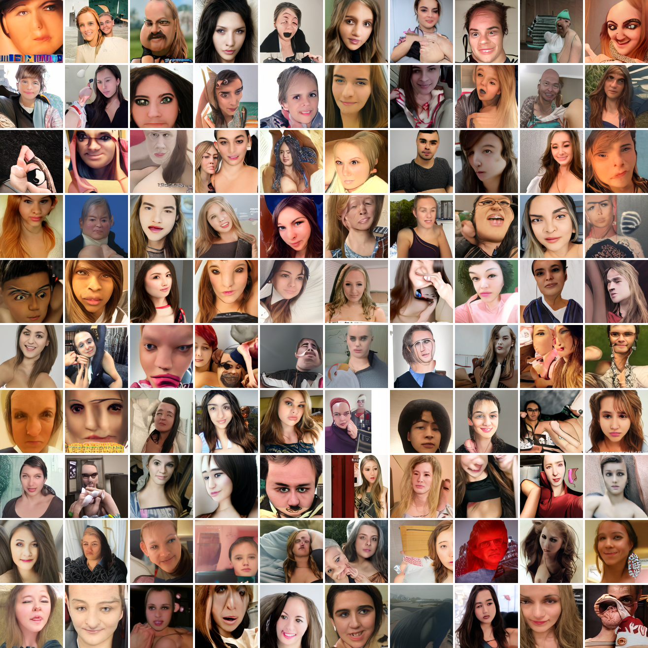
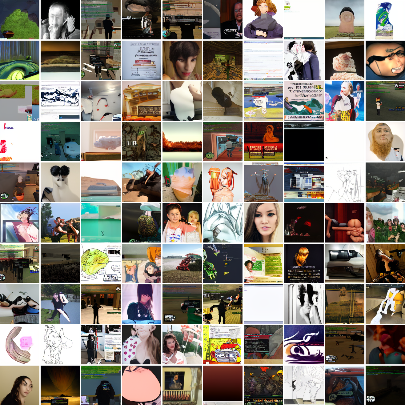
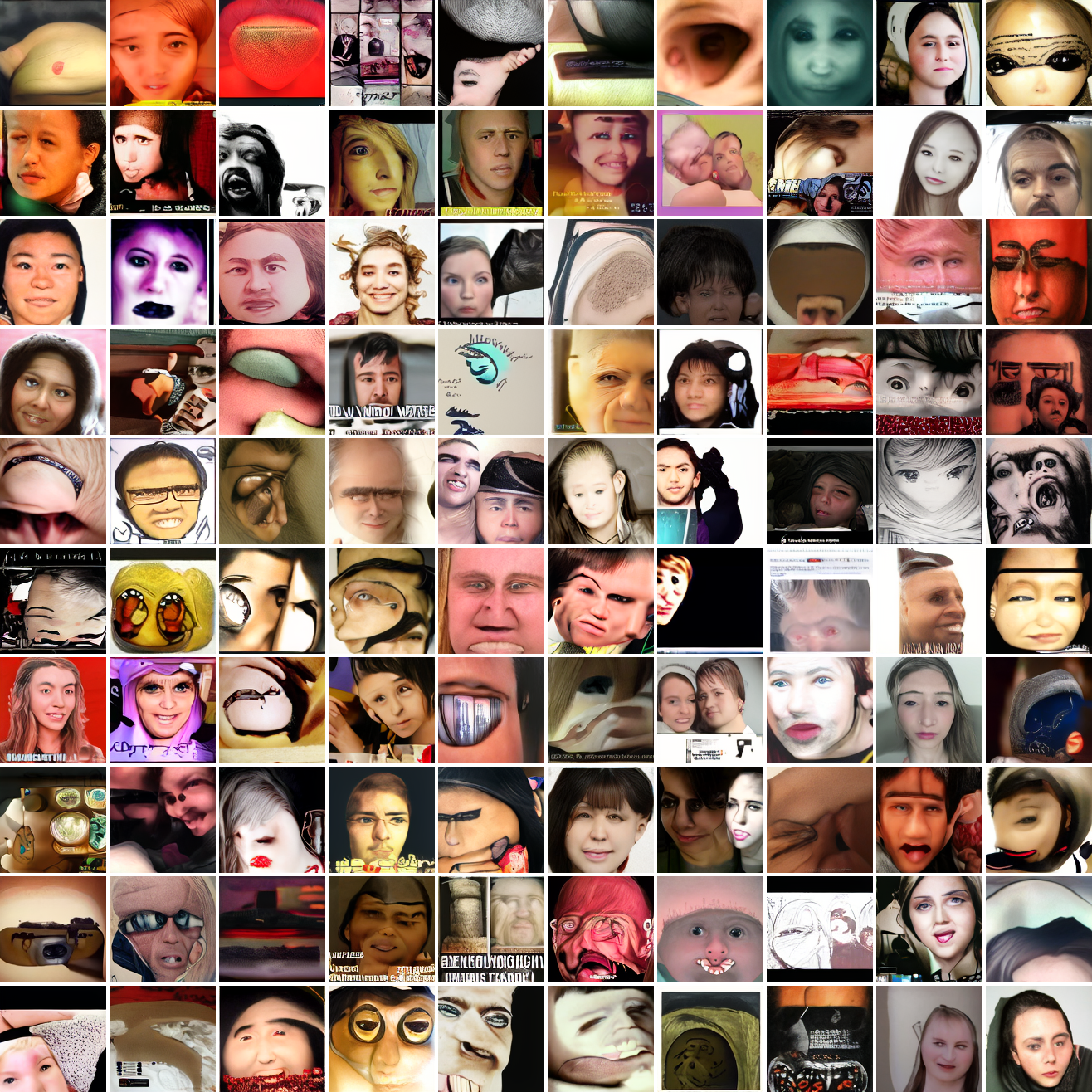
Let’s try the text prompts I used with the baseline model. Here’s “A woman’s face”:
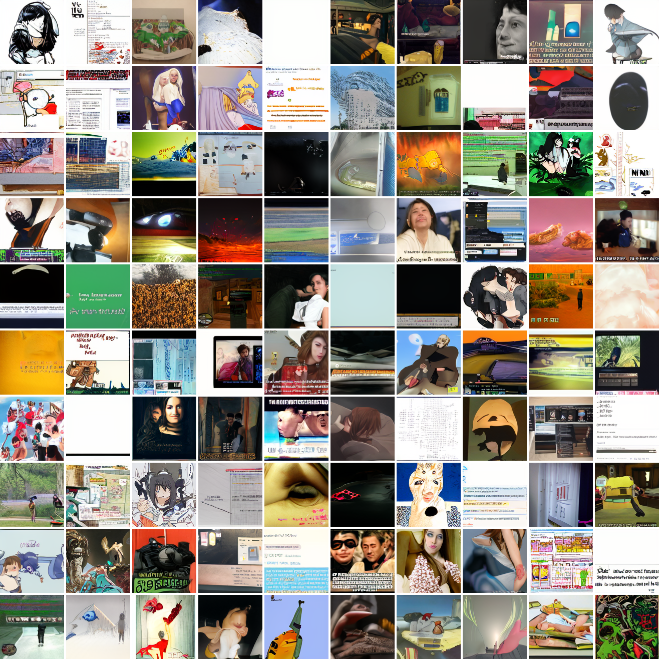
Here’s “a screenshot of Grand Theft Auto”:
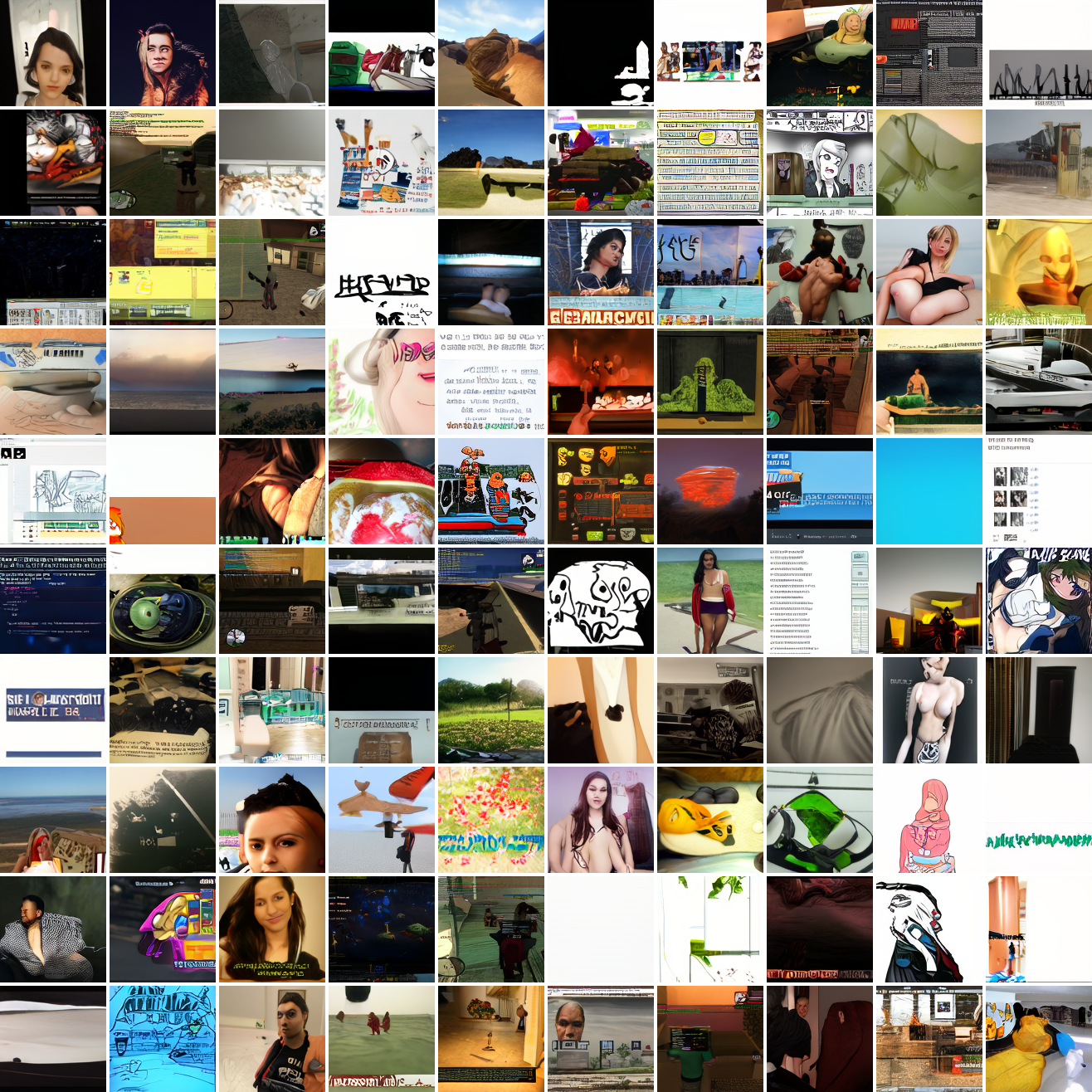
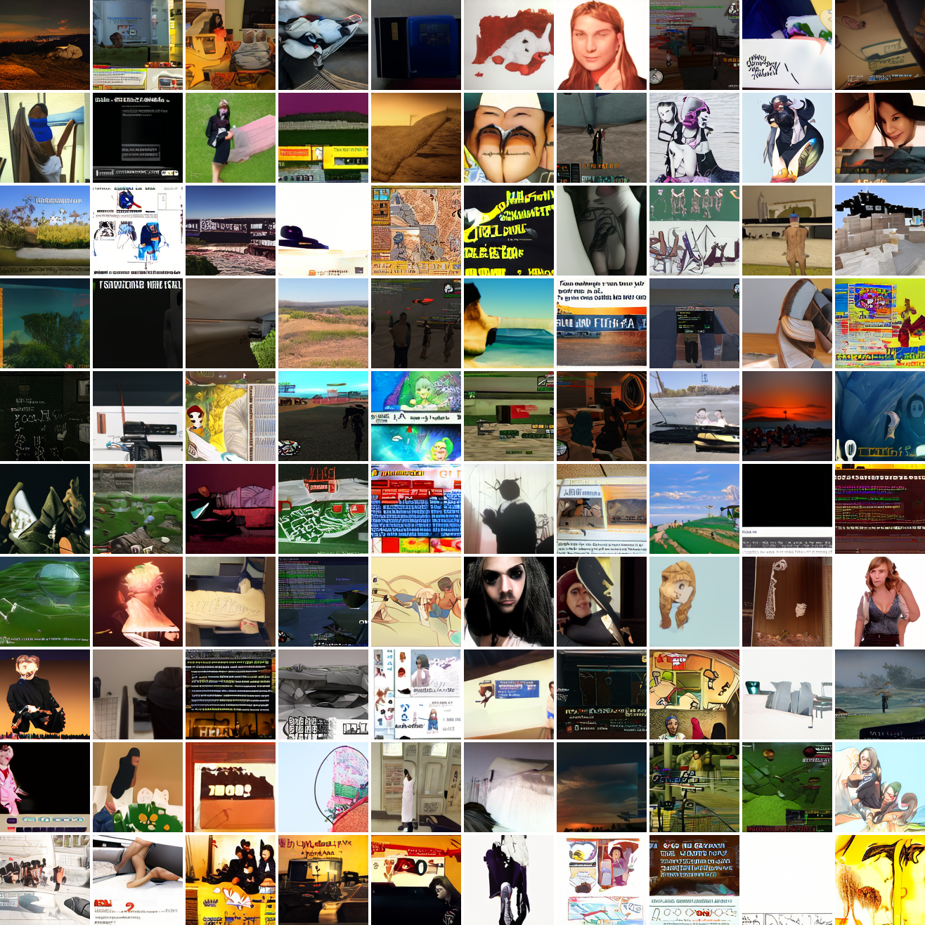
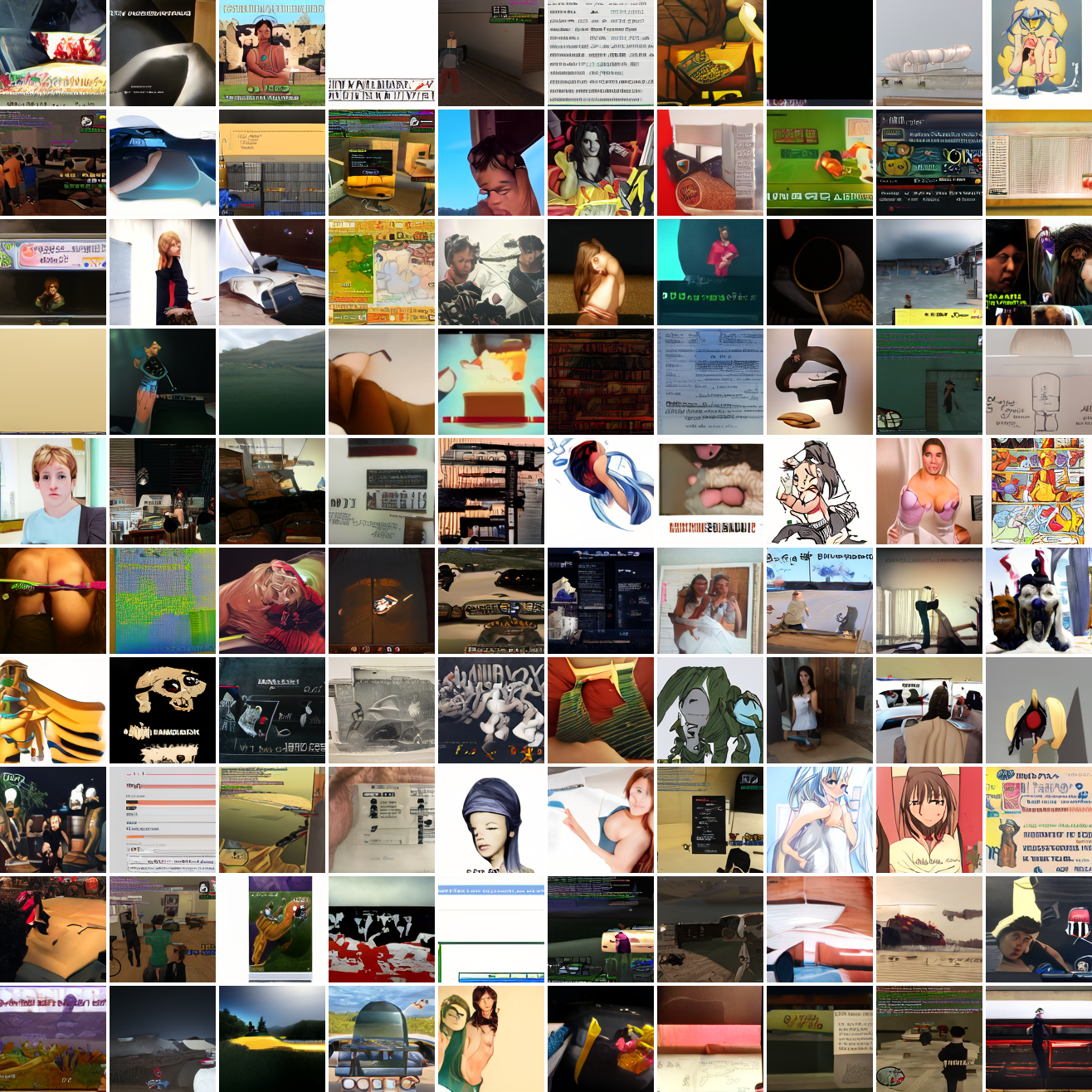
In both cases the fraction of images that resemble the prompt increases as the max cosine distance decreases. In the case of faces, there are high numbers of images that have faces in the range of 0.0 to 0.6 maximum cosine distance, but in the case of GTA screenshots, the range is more like 0.6 to 0.7. This makes some sense: the baseline model successfully generates faces when given an appropriate text prompt, but it can’t generate GTA screenshots from one. So we can suppose that there are images that have the same embedding as the text “A woman’s face”, but there aren’t images that have the same embedding as the text “A screenshot of Grand Theft Auto”. The cap conditioned model can only produce images that have embeddings inside a given cap if those images exist in the distribution.
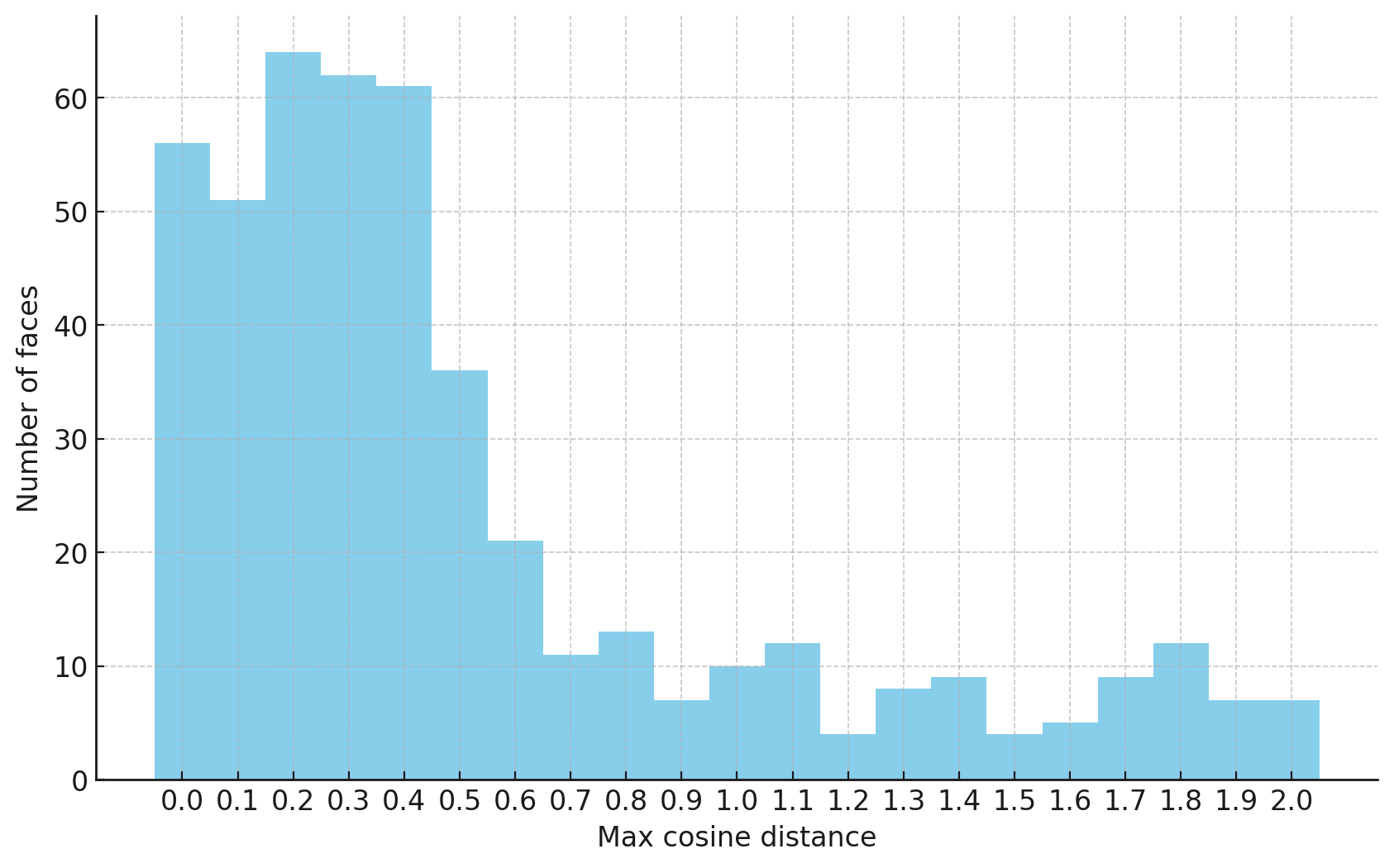
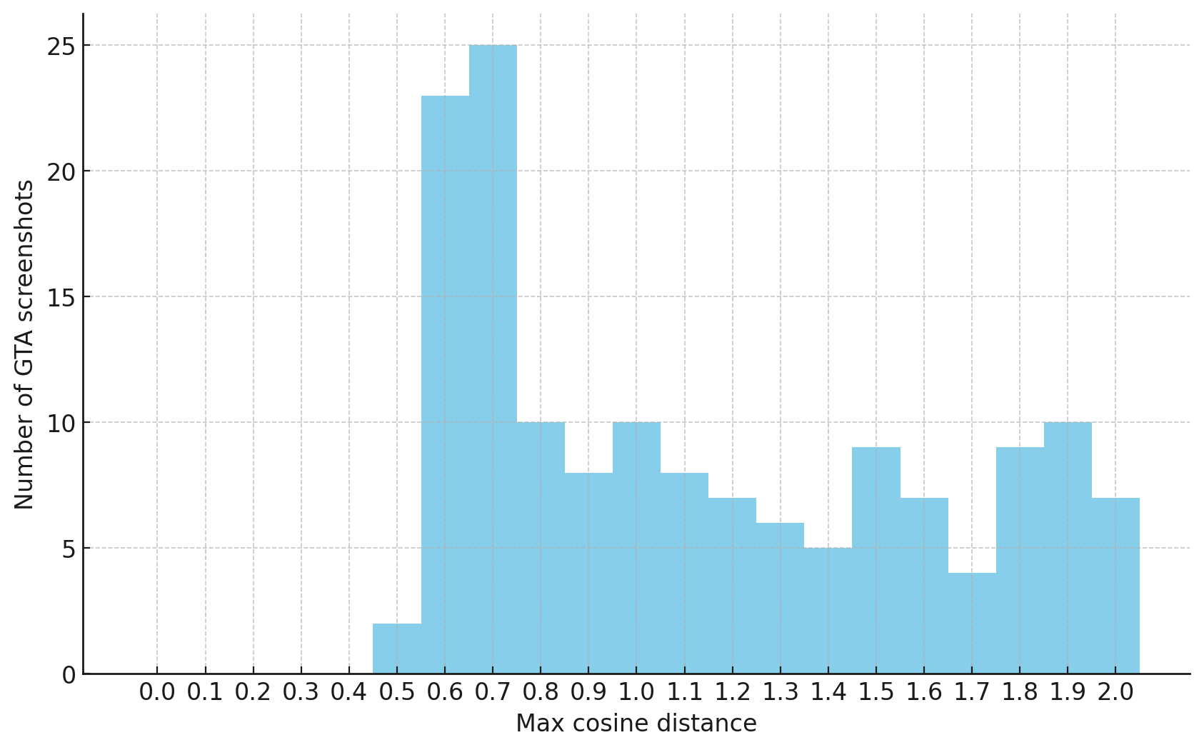
The fraction of the images that resemble a GTA screenshot never exceeds 25%, and the fraction with faces never exceeds 64%. The model is undertrained, but I think this is actually decent proof of concept.
Next steps
Given all this, I’m reasonably confident this approach is sound. But as you saw in the samples, it doesn’t work very well yet. The simplest thing to do is scale up, training the model for longer, perhaps going up another notch in model size. It’d be much better to generate more cap-image pairs than to train for more epochs with the exact same pairs. And getting more data is of course always good. But I’ve seen very impressive results using comparable amounts of data to what I’m working with (the PixArt- guys brag about 33M), so that’s less of a priority.
Aside from model scale, I think it’d be worth messing with weighting the loss. The cap conditioned model mostly ignores the conditioning data at higher max cosine distances, and has similar loss to the baseline model, so I’m pretty sure that it’s mostly learning the unconditional distribution - predicting later image tokens from earlier ones and not from the conditioning token. It’s possible to counteract this by weighting the loss so that earlier tokens - where’s there’s less information from the image tokens and more from the conditioning token - are weighted more heavily. Worth experimenting with.
Another thing likely to improve quality is some kind of dataset balancing. It’s way too good at GTA screenshots relative to other stuff, and this is because they’re massively overrepresented in the dataset. On the other hand, it’s not that great at them so maybe better balancing would just get me a model that’s bad at everything.
This is a simplification. In reality, at each training step, there are n images and their n captions. The cosine similarities between each image’s embedding and each caption’s embedding are computed, then fed into a softmax, after a scaling factor is applied. The objective is to minimize cross entropy loss, and the scaling factor is learned. Anything I do with CLIP ignores the scaling factor and the softmax.↩︎
Both models are decoder only transformers generating 128x128 images, trained for one epoch on the 25 million image subset of my Imgur dataset that are sufficient resolution and are in RGB. The conditioning data is prepended to the sequence as a special token. The models generate sequences of 1024 tokens, which are fed into an autoencoder adapted from Latent Diffusion, which I ported to Jax/Flax, reusing their weights. The models use the middle size hyperparameters from the GPT-2 paper - 36 layers, d_model 1280, total parameters ~543M. The GPT-2 paper lists 762M in that configuration, and some of the difference is accounted for by the difference in vocabulary size (8192 vs 50,257). I’m not sure about the remainder. All samples are generated with top-p filtering with p=0.9. Models are trained with bf16 activations and f32 weights, and sampling is done with f32 activations.↩︎
Gathering A Dataset of 33 Million Unlabeled Images from Imgur
As part of a machine learning project to build a text-to-image model, I gathered a large dataset from archives of Imgur. Well, 33 million images in around 11 terabytes sounds big to me, but there are people out there that probably ingest that much in a day. 🤷♂️ For my purposes, it’s enough for proof of concept. Anyway, there’s some interesting stuff about the dataset, and some of the work I did to gather it, so I thought I’d write it up.
The archives
In April 2023, Imgur changed their terms of service and announced that they would be deleting “old, unused, and inactive content that is not tied to a user account” and “nudity, pornography, & sexually explicit content” on May 15. This prompted Archiveteam to start a project to archive as much of Imgur as possible given the remaining time. Imgur launched in 2009 and hosted a ton of images which are linked all over the web. Turning all of those into 404s would be something of a tragedy. Archiveteam exists to avert tragedies like those. If someone is deleting a public resource they go and preserve it. Anyway, I heard about what was going on, got to thinking, and ran their archiver software on my machine for a while. Everything grabbed by anyone running the archiver gets sent to Archiveteam for processing, and eventually ends up on the Internet Archive, in a big pile of archives. I think it ends up in the Wayback Machine later, but I don’t really understand the whole process.
To gather my dataset, I downloaded, processed, and stored 1,332 archives from the pile. As of writing there are 49,731 total archives in there, with an average size of 14 GiB, taking up around 680 TiB. A lot of that is redundant - my processed archives are on average 10.24 GiB. That’s after removing downscaled copies of the images, deduplicating by hash, and generating a still from every video. Based on the number of images in my archives, I estimate the total number of unique images in the pile to be around one billion.1 Far more than the 33 million I’m working with. Part of the appeal of this dataset is that it’s effectively infinite. Once I’ve written the processing code, getting more data is a matter of spinning up a VM and running it for a few days. Fetching from IA isn’t fast, but if your alternative is downloading from the web in general like you would if you were grabbing LAION-5B, it’s pretty good.
My title say 33 million, but the actual number of usable images is ~25 million in the context of my project. My preprocessing (which runs after the processing and before the other processing (with an optional processing step in between)) script drops everything smaller than 128x128, everything that’s not RGB, and everything that Pillow can’t load.
What’s in there?
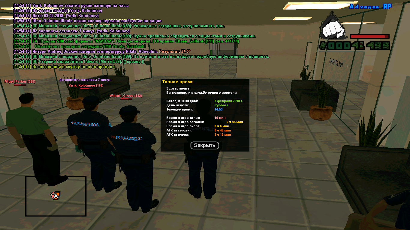
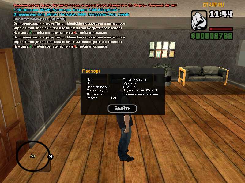
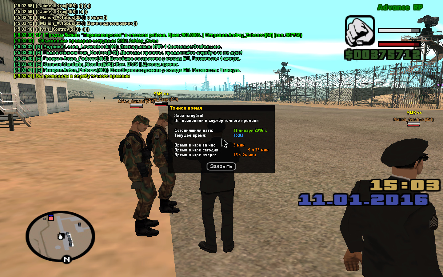
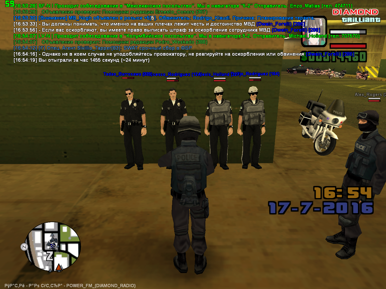
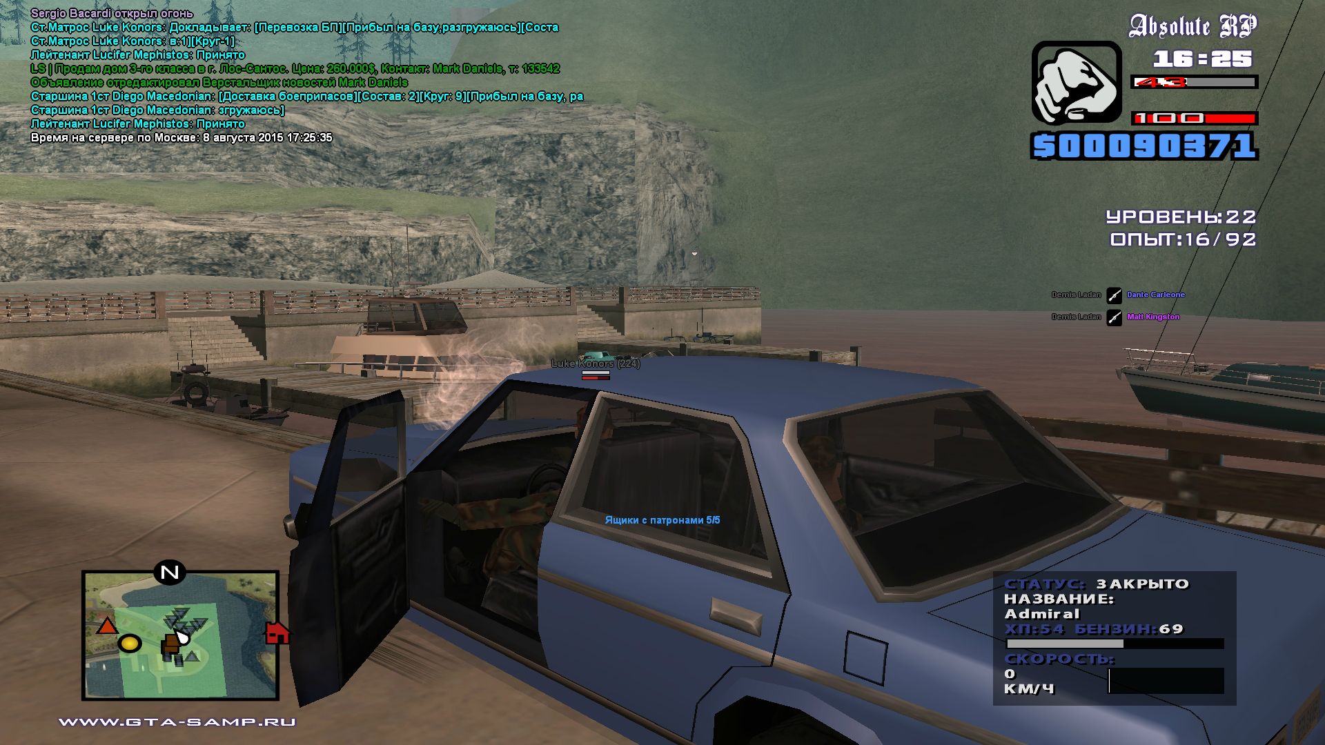
Tons and tons of screenshots of GTA. Seriously, it’s absurd. Why were people uploading so many screenshots of GTA to Imgur? Someone please tell me. It’s around 9% of the dataset, around as much as all the other video games combined.
I made a little gallery you can take a look at, based on a sample of 5000 images from the dataset. Take a look. I manually tagged all the NSFW images, and they’re filtered out by default. There are radio buttons at the top to turn that off or invert it if you’re curious. That said, there’s still plenty of objectionable stuff in there, including at least one Happy Merchant and a use of the “N word”.
As you can see, it’s far from a representative sample of all the pictures that exist, or all the pictures that were ever uploaded to the internet. Imgur has a particular userbase, a particular usecase, and the images that Archiveteam’s efforts grabbed are non-representative as well. To speculate, the images archived are probably biased towards images that were more likely to be deleted, more popular among the sorts of people that upload lists of images to be queued for archiving, and more likely to be linked in places that were scraped for links.
Some broad categories of images:
- Screenshots of GTA
- Screenshots of other video games
- Comics
- Memes
- Screenshots of websites
- Anime
- Pornography and titillating non-pornography
- White on black Russian text
- Labels for Russian standardized exam videos?
- Just says “download link” with some number
- As best I can tell there are (were) some Russian people who used Imgur to store images used as titles for stuff?
- Pictures of English text. Outside of screenshots this is less common than Russian.
I don’t mean to imply that these are the only types of images in the dataset, just that their prevalence is striking when you look at it. Spend a few minutes scrolling through the gallery and you’ll see what I mean. If I look at the first 16 images in a shuffled gallery I see: a photo of the box and disc of a video game, a photo of a watch, a nature photo of a beach, something unrecognizable, some weird meme, a picture of Nelson from the Simpsons, a sprite sheet I think, a photo of a guy in a beanie, a nude photo of a man, a pro wrestling promo image, a screenshot of GTA, a screenshot of Google Image Search results, what looks like a screenshot of Minecraft, some microelectronics work in progress, an album cover, and another screenshot of GTA.
I went through 140 images and did some quick stats:
- 32% have at least one woman in them
- 39% have at least one man
- 4% have nudity
- 9% are screenshots of GTA
- 11% are screenshots of other video games
A lot of the images with men are screenshots of games. Excluding those, 30% had at least one woman, and 24% had at least one man. On the other had, of the images with nudity, 71% had at least one woman and 43% had at least one man. A great deal of the overrepresentation of women is due to pornography as well as pictures of women in titillating poses and outfits. This might lead to an image model using the dataset being more likely to draw women nude, and it would almost certainly lead to one being better at drawing nude women than nude men, but I won’t draw firm conclusions before seeing results from an actual model.
As an aside, ChatGPT-4 is quite good at answering “wtf is this picture?” type questions. The vision model is capable of photo OCR and the language model can do translation, along with understanding a ton of shit.
Data gathering automation
I wrote a bunch of automation, but honestly most of it isn’t too interesting to anyone else. A few highlights:
- Untarring and tarring things can be a bottleneck with a real disk. Getting a machine with a ton of RAM and making a huge tmpfs solves this.
- If you pipeline it so that downloading, processing and uploading can happen simultaneously you can get big performance gains. At the cost of having to debug concurrency issues.
- Some hash functions are faster than others. Use BLAKE2b.
- As always, the right indexes are essential to making SQL fast. You can put the things in the
WHEREclause of your query in theWHEREclause of your index. - Cloudflare’s R2 is substantially cheaper than S3.
I’ve processed and uploaded 1,332 archives, containing a total of 32,945,613 unique files. That’s ~24,734 files per archive. That times 49,731 makes 1.23 billion files. This is probably an overestimate, since the more archives you’ve seen the more likely an image in a new archive is to be a duplicate. So I’ll ballpark it at a billion.↩︎
JAX vs PyTorch: A simple transformer benchmark
I’ve been looking into deep learning libraries recently and JAX seemed interesting, but as far as I could tell no one had actually benchmarked it against PyTorch, the de facto standard. So I decided to implement the same model in both and compare. Here’s the top level summary: PyTorch gets 1.11 iterations per second and JAX gets 1.24it/s (12% better) on a Google Colab notebook with a P100. In addition, JAX is more memory efficient, the PyTorch model OOMs with more than 62 examples at a time and JAX can get up to 79 (at 1.01it/s, or 79.79 examples per second vs PyTorch’s 68.82 with the smaller batch size).
Meanwhile TPUs are kind of absurd. Torch on XLA theoretically exists, but I don’t know of anyone who’s actually gotten it to work. When I was testing it my code segfaulted. TPUs work very smoothing with JAX though. I was accepted in the TPU Research Cloud (formerly TFRC), and a TPUv3-8 can run through 2,591 examples per second with a batch size of 3,032.
Benchmark details
You can reproduce my GPU results using this notebook and find the model code here. The TPU code is in the pmap branch. Unfortunately Colab TPUs are flaky so there’s no notebook for that. The model is a simple, byte-level, autoregressive transformer language model trained on enwik9. I used the Flax neural net framework for the JAX implementation. The hyperparameters are as follows:
| Parameter | Value |
|---|---|
| layers | 12 |
| d_model | 512 |
| heads | 8 |
| feedforward dimension | 3072 |
| sequence length | 256 |
It’s GPT-1 with embedding dimension 512 instead of 768. Quite small in comparison to SOTA models.
Caveats
This is, obviously, a single measurement. The comparison, and the direction of the advantage may vary by model type, size, hardware, and other factors. I’m not making any universal statements here. Furthermore, 12% better performance isn’t much. Competent ML engineers are expensive (and your time is valuable) - it’s easily possible that you lose more in engineering time than you gain in training time. And it’s always possible I’ve made a mistake and the two models aren’t actually identical.
Observations about programming in the two systems
I haven’t done a ton of ML programming in either Torch or JAX/Flax, but I can compare what I do know of them.
- Torch is much more batteries-included. There’s a
TransformerEncoderand aTransformerEncoderLayerintorch.nn. In Flax, there’s an attention module, but the transformer assembly - attention + feedforward + layer norm + residuals - I had to write myself. vmapis very cool. Briefly,vmapallows you to turn any function into a vectorized version, and JAX will generate efficient code for you. So I could get rid of batch dimensions everywhere except the outermost layer, and give myself one less thing to get wrong.pmapis very cool too. Analogous tovmap, it lets you parallelize code across multiple accelerators and across multiple host machines, provided the accelerators have a special cluster setup for fast interconnect. In practice I think that mostly means TPU pods, though they do mention a way to do it with Nvidia GPUs.- TPUs are really really powerful. Good TPU support, especially since I have access to TRC, makes the choice easy.
- All the indirection that Flax introduces to let you write models in an object oriented style makes the stack traces really bad. They’re like 80% stuff internal to Flax or to JAX’s JIT.
- JAX’s approach to differentiation is more powerful and less footgunny than Torch’s. It’s not possible to accidentally compute useless gradients or accidentally modify things that shouldn’t be learned parameters.
- Performance debugging is easier with Torch. If you use the profiler on a JAX program, everything that’s been JIT compiled shows up as “custom-call” or “fused”, and the JIT compiled code is all of the code who’s performance you care about. Apparently it works if you use the special secret profiler Google has internally.
- Being a much less used library, it’s much harder to Google error messages and the like.
Conclusion
I like JAX, and I intend to use it for my next big project (a CLIP conditioned image generation model). But if TPUs and especially the TRC didn’t exist, I’m not sure it’d be worth it.
Samples
I let the model train for around four days on a TPUv3-8. I was surprised by how well it works. Note that Wikipedia uses triple single quotes for bold and double single quotes for italics. All article ledes include the subject in bold.
| Prompt | Sample |
|---|---|
'''Star Trek''' |
'''Star Trek''' is a fictional [[supervillain]] of a [[fictional character]], a male [[antagonist]], and a supervillain of a supervillain [[animation|animated]] [[science fiction]] [[television series]]. One time writer [[Andrew Stewart]] used Star Trek to |
'''Star Trek''' |
'''Star Trek''''') is a [[comic book]] series continuing as a new [[1990s]] and [[1992s]] [[comic book]] character from [[Tony Straight]]. It is one of the oldest programs in the series, played by the [[Halloween]] television series ''[[Doctor Who]]''. The |
'''Star Trek''' |
'''Star Trek''''' is a series of series produced by [[Wizards of the Coast]] featuring several stories and endings. These combine to form the novel ''[[What's New, Purgatory?]]'' and its musical numbers. ''[[The Whales of Magellan]]'' is a [[science fictio |
'''Star Trek''' |
'''Star Trek''' or '''Kazna''' which literally means "childhood canal". Star characters were either [[warp drive]]s or [[computer-generated imagery|scale control video]]s are the primary weapons in the series. The series was premiered in [[2002]] |
'''San Francisco''' |
'''San Francisco''' is the name of many attractions situated on [[San Francisco International Airport]]. It is one of the few free airports located near [[Panama City, Florida]].== History ==Stanford was founded in 1918 as the home of The San Francisc |
'''San Francisco''' |
'''San Francisco'''. After the [[Mexican-American War]] the seaport developed into the seat of the city of [[Rio Grande, California|Rio Grande]]. Passenger service was directed to [[New York City]] by surveyor San Francisco Parks Corporation. The passenger |
'''San Francisco''' |
'''San Francisco''', named after the San Gabriel [[mariage]] and [[Irish Catholic]] [[eschatology]] founded in 1863 by San Gabriel (Redfern) was named in honor of ''Cestion San Francisco'' (a term which the reputed early mariage was held up by [[Native Ame |
'''San Francisco''' |
'''San Francisco''' (born '''Mark Antonio Baldwin''' [[September 2]], [[1945]]) is a [[Canada|Canadian]] [[Public house|pub]] owner and legend of [[Uburban Culture]] [[Public house|pubs]].Baldwin started his own business in [[1963]] when he left to sett |
'''George Walker Bush''' |
'''George Walker Bush''' (born [[July 13]], [[1954]]) is an [[United States|American]] [[physicist]] and [[Nobel Prize]] winner. He was born in [[Albany, New York]].Born '''George Lauder-Freiherr Bush''' (born [[March 10]], [[1957]]) he became a member o |
'''George Walker Bush''' |
'''George Walker Bush''' (born [[July 7]], [[1961]]) is an American [[philanthropist]] who at one time secured a record of 3 works before attending the [[Carnegie Institute of Technology]] and became a full-time journalist in [[1994]].Born in [[Frankfor |
'''George Walker Bush''' |
'''George Walker Bush''', [[United States Republican Party|Republican]] ([[Democratic Party (United States)|Democrat]])* '''George Mills''', [[United States Democratic Party|Democrat]] ([[Democratic Party (United States)|Democrat]])* '''[[Anthony Burrows |
It doesn’t seem to know what Star Trek or San Francisco are, or who George W Bush is, but it does associate Star Trek with nerdy entertainment, television, and warp drive. Similarly, it associates SF with SFO, Stanford, and California. It seems to know, at least sometimes, that George W Bush is associated with US politics as well. And it’s learned what the ledes to biographies look like.
CommentsPrediction results for 2017
I made 35 predictions last January, and judgement day has come. Well, technically is was the 1st, but I’m writing this today. I’ll use evidence as of the 1st where possible. I’m inverting some of them so all the predictions are ≥ 50%.
Politics
- Trump takes office on inauguration day: 95%.
- TRUE. This one was pretty obvious. Maybe low.
- Trump is not impeached: 85%.
- TRUE. Maybe low? Impeachment takes a long time.
- Trump is not murdered nor does he survive an attempted murder: 95%.
- TRUE. Wikipedia There have been 31 attempts in American history, successful or not. The presidency was established March 4th 1789, and there are 83,231 days between that and January 19 2017. So a rate of 3.766249544405297e-3 per day. There were 346 days between January 20 2017 and January 1 2018. 1 - ((1 - 31/83231) ^ 346) gives us a 12.09% probability of assassination. So I think this one was high, especially accounting for how unpopular he is.
- Construction on US-Mexico border wall doesn’t begin: 80%.
- TRUE.
- ACLU launches at least one major lawsuit against new federal policy: 90%.
- TRUE. This might’ve been low.
- No mass deportation program begins: 80%.
- TRUE. Politifact says deportations are actually down though that may be an artifact of how they’re tracking. Regardless, nothing that qualifies as “mass”.
- Trump’s approval rating as reported by Gallup is below 45%: 65%.
- TRUE. Gallup’s website is kind of awful, but they had him at 40% approve 55% disapprove on December 30th.
- The US doesn’t uses a nuclear weapon on a populated area: 95%.
- TRUE.
- Legislation requiring the weakening/backdooring of cryptography and/or computer systems in general is not passed in the US: 75%.
- TRUE.
Technology
- Someone writes a web framework for Idris: 65%.
- FALSE. There already was one, last updated in 2014.
- Conditioned on my going back to work on it, Idris gets a new build system: 90%.
- INVALID. I didn’t go back to work in it.
- I go back to work on it: 65%. (I make no estimate on whether anyone else will rewrite it)
- FALSE. Early in the year I switched my projects to stuff that seemed more likely to get me a job, and later in the year I was working and develpoed pretty bad RSI.
- There are at least two more papers published about/using Idris: 90%.
- TRUE. Two by Edwin Brady alone: Type-Directed Reasoning for Probabilistic, Non-Compostitional Resources and Automatically Proving Equivalence by Type-Safe Reflection. Almost certainly more.
- No program written in Idris gets substantial use outside of the Idris community: 90%.
- TRUE. AFAICT anyway. Happy to be proven wrong.
- There are at least 36 jobs found when searching for Haskell on Stack Overflow Jobs. (18 at time of writing): 75%.
- FALSE. It’s 17 as of time of writing. Haskell seems to be getting less popular over time, which really doesn’t bode well. I’m not sure how to explain the trend. Stack Overflow trends.
- There are at least 30 jobs found when searching for Tensorflow on Stack Overflow jobs. (7 at time of writing): 75%.
- FALSE. 19 at time of writing.
- There will be at least one large breach of user data reported at Yahoo, Facebook or Google/GMail: 80%.
- FALSE.
Personal life
- I will be living in a different house: 85%.
- TRUE.
- I will be living in a different metropolitan area: 65%.
- FALSE.
- I will have a job programming: 80%.
- TRUE.
- I will have any job at all: 95%.
- TRUE.
- I will have more average positive social interaction per time, excluding work: 80%.
- Hard to tell. Not substantially up for sure.
- My weight will be less than or equal to 180 lbs: 70%.
- FALSE. I’m was at 224.8 as of January 1. I’ve started a new weirdo diet as of the 13th which is working, so this might be improved next year.
Personal work
- PDXFunc attendance will increase at least 50%: 75%.
- TRUE. 90%+ of the credit for this goes to Lyle.
- I will publish software written mostly or entirely by me, outside of work, that has at least 5 users: 85%.
- FALSE. Beescheduler has 1 active user (hi!). A bunch of people signed up and then completed their goals, although I don’t actually know if they deauthorized the app before that.
- The software quality survey will be online or completed: 80%.
- FALSE. Same reason as the Idris stuff above.
- The collection of explanatory variables for the software quality study will have begun: 70%.
- FALSE. These are all counted as in addition to the above, not conditional.
- I will have published conclusions from the study: 50%.
- FALSE.
- I will not have published conclusions that are valid and actionable: 65%.
- TRUE.
- No one other than me will take them into consideration: 87%.
- TRUE.
Media
- No full length Half-Life game will be released: 95%.
- TRUE. We did get some nice prose from Marc Laidlaw though.
- No announcement of same: 70%.
- TRUE.
- Steven Universe is still airing: 85%.
- TRUE.
- At least one gameplay patch for Dota 2: 90%.
- TRUE. There were 14 in 2017.
Analysis
My cross entropy score was 0.807 (range 0 - infinity), my Brier calibration was 0.0204 (range 0 - 1), my Brier refinement was 0.1496 (range 0-0.25) and my overall Brier score was 0.1701 (range 0-1). For all of those metrics, lower numbers are better. I was overconfident for the buckets from 50% to 85% and underconfident for 87% to 95%. Here’s a calibration chart: 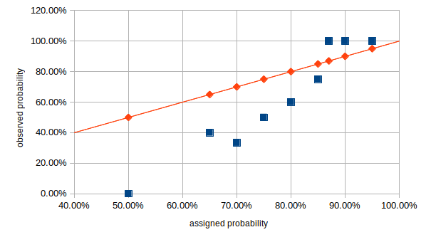
The red line is perfect calibration, my buckets are in blue.
I’m not really sure what lessons to draw from this. In future, I’m not going to do this on a yearly basis - it’s much better to get feedback quicker and more often that once a year. I may start using PredictionBook, though annoyingly they compute Brier scores but not the decomposition into components.
Technology was my worst category by cross-entropy - 1.3793. The breach prediction and the jobs predictions were worst. In the TF jobs one I was very overconfident. There are a lot of postings for the `machine-learning tag, but not for TF specifically. I think I overestimated how much employers care about specific libraries and how complicated industrial ML work is. The Haskell prediction I talked about above.
My second and third worst were the personal categories. I was overoptimistic about project difficulty, succumbing to the planning fallacy even though I’m supposed to know better, and I underestimated how much time and energy professional work would take up. Which is not to say it was a bad year, I really like my job. My RSI seems to be getting better so perhaps I’ll be able to spend time on personal projects in 2018.
CommentsPredictions for 2017
Here are my predictions for 2017, such as they are. The idea is to develop the skill of prediction by making and testing them somewhat regularly. I don’t expect to do super well.
Judgment date is January 1 2018.
I’m aiming mostly for calibration, but will also compute cross entropy.
Politics
- Trump takes office on inauguration day: 95%.
- Trump is impeached: 15%.
- Trump is murdered or survives an attempted murder: 5%.
- Construction on US-Mexico border wall begins: 20%.
- ACLU launches at least one major lawsuit against new federal policy: 90%.
- Mass deportation program begins: 20%.
- Trump’s approval rating as reported by Gallup is below 45%: 65%.
- The US uses a nuclear weapon on a populated area: 5%.
- Legislation requiring the weakening/backdooring of cryptography and/or computer systems in general is passed in the US: 25%.
- I was going to put something about political partisanship here, but I can’t find a survey that happens regularly enough.
Technology
- Someone writes a web framework for Idris: 65%.
- Conditioned on my going back to work on it, Idris gets a new build system: 90%.
- I go back to work on it: 65%. (I make no estimate on whether anyone else will rewrite it)
- There are at least two more papers published about/using Idris: 90%.
- A program written in Idris gets substantial use outside of the Idris community: 10%.
- There are at least 36 jobs found when searching for Haskell on Stack Overflow Jobs. (18 at time of writing): 75%.
- There are at least 30 jobs found when searching for Tensorflow on Stack Overflow jobs. (7 at time of writing): 75%.
- There will be at least one large breach of user data reported at Yahoo, Facebook or Google/GMail: 80%.
Personal life
- I will be living in the same house: 15%.
- I will be living in the same metropolitan area: 35%.
- I will have a job programming: 80%.
- I will have any job at all: 95%.
- I will have more average positive social interaction per time, excluding work: 80%.
- My weight will be less than or equal to 180 lbs: 70%.
Personal work
- PDXFunc attendance will increase at least 50%: 75%.
- I will publish software written mostly or entirely by me, outside of work, that has at least 5 users: 85%.
- The software quality survey will be online or completed: 80%.
- The collection of explanatory variables for the software quality study will have begun: 70%.
- I will have published conclusions from the study: 50%.
- The conclusions will be valid and actionable: 35%.
- Anybody other than me will take them into consideration: 13%.
Media
- No full length Half-Life game will be released: 95%.
- No announcement of same: 70%.
- Steven Universe is still airing: 85%.
- At least one gameplay patch for Dota 2: 90%.
One of the Best Decisions I've Ever Made: Beeminder
Starting to use Beeminder late in 2015 is, no exaggeration, one of the best decisions I’ve ever made. I’m much happier and have gotten much more done than I ever did before. I’m gonna be cute and call it Willpower as a Service. If you ever procrastinate or don’t do things you know you should, I highly recommend it.
Here’s how it works: you set a goal to do something and a rate at which you want to do it. Whenever you do it, you type how much you did into the site. If you don’t do it, they charge your credit card. You can decrease the rate or quit whenever you like, but it’s always delayed a week from when you do so.
Whenever I tell someone this, they laugh. It’s sounds ridiculous, but it’s amazingly effective. What it does is turn long term desires into short term ones. For example, I have a goal to work on projects that will make me more attractive to employers 20 hours a week. (It used to be working on Idris, but I wasn’t getting enough interviews.) I also have a bicycling goal (5 miles/wk) and one working on my software quality causes project (10 hrs/wk). To paraphrase Dorothy Parker, I hate programming, I love having programmed. I enjoy solving problems, it’d be satisfying to improve the state of programming languages and getting the respect of my peers is great, but those rewards are all intermittent and far in the future. Most of the time it’s a slog. When the work is boring and frustrating it’s much easier and more fun to just fuck off and watch Netflix all day. Beeminder turns my long term desires into short term ones. I could watch something instead of working, but it’d cost me 30 bucks. A month into the future, I’m much happier if I worked on my projects than if I rewatched The West Wing for the billionth time.
It also features extremely satisfying graphs: 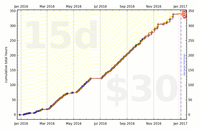
It’s really really satisfying to see all the work you’ve done.
This post isn’t sponsored or anything, I just think you might benefit from it.
CommentsAnnouncing AlanDeniseEricLauren, an implementation of the ADEL algorithm
I uploaded AlanDeniseEricLauren to Hackage today. Here’s the README:
AlanDeniseEricLauren is an implementation of the ADEL algorithm for efficiently finding the minimal subset of an input set satisfying some arbitrary upward-closed property. “Upward-closed” means if the property is true of some set S it is true of all supersets of S. My implementation is trivially extended to maps (dictionaries).
This can be used for e.g. narrowing down bugs by finding the minimal subset of a complex failing test case that still exhibits the issue. In addition, I provide a method for finding the minimal set of changes between a known-good and known-bad example needed to trigger a bug. (Equivalently, a set where the property is false and a set where it’s true.)
The ADEL algorithm is due to Philippe Laborie in his paper “An Optimal Iterative Algorithm for Extracting MUCs in a Black-box Constraint Network” published in ECAI 2014. doi:10.3233/978-1-61499-419-0-1051. The paper is available at http://ebooks.iospress.nl/publication/37115.
The project’s homepage is https://github.com/enolan/AlanDeniseEricLauren. Bug reports and PRs can be submitted there.
As of August 2016, I am looking for work. If your company needs a good programmer, my email is echo@echonolan.net. My resume is available here.
CommentsNotes toward an empirical study of programming language effectiveness
I’ve decided to do an empirical study of the effects of programming language choice. As a PL enthusiast, I’d like to know what languages are actually helpful in practice and whether the ones I like are actually any good. The existing research is, well, not great. In this post, I’ll describe my current thoughts. If you have feedback on the design, please leave a comment - I make strong statements below, but I’m sure I’ve gotten some things wrong. If you’re interested in collaborating, get in touch too. This is big and complicated and I’d love to work with others on it.
A randomized controlled trial would be nice if I had infinite money and time
An observational study is the only way to go. Experiments need to use trivial tasks and small n or are unfeasibly expensive, even if I had institutional backing. Consider a typical software project: we’re talking hundreds of person-hours over a period of at least months. Projects done in a lab over a few days aren’t similar enough to be comparable. Readability, types, testing, documentation, etc matter much less when it’s all fresh in your mind and you don’t have to explain it to anyone. Refactoring is unlikely to happen at all. Let’s make up some numbers: a smallish project over three months with three developers working full time. We’ll assume they’re cheap and put them at $24/hr (the 25th percentile) . $24/hr * 40hrs/week * 4 weeks/month * 3 months * 3 developers is $34,560. Per case. For a sample size that gets you significance we’re talking hundreds of thousands to millions of dollars. Maybe more, since I expect the outcome standard deviation to be high.
Given the decision to do an observational study i.e. collect data on projects that already happened, we need to control for confounders. Confounding variables aside, collecting anything that influences outcomes will give us more accurate predictions and allow us to detect smaller effects. The easy/obvious ones are project age, start year, team size, topic area, commercial vs noncommercial and company age at project start. It’d be best if I could also measure team skill but I don’t have a test for that and even if I did I couldn’t administer it. Experience level would be a decent proxy but I also won’t be able to measure that. I just have to have to hope the measurable stuff is an adequate proxy. There are probably some I’m missing.
How to judge outcomes
People make various claims about what advantages various programming languages have. Java is good for large enterprise projects, Ruby lets you get something working fast, C lets you write fast programs, Haskell makes it harder to write bugs, etc, etc. In the interest of simplicity I’ve decided to skip anything more precise than user satisfaction. Everything else is difficult to measure consistently and only instrumental to the actual point of the software. I know it’s weird that I’m advocating a subjective measure in the interest of consistency, but more specific things like bug rate, performance and feature count are subjective too and difficult to compare across projects and categories. What counts as a bug? Is this one bug or five? Is this rendering engine faster than this compiler? Is CSS3 support one feature or lots? Etc.
So we’ll survey users. “Have you used a program that’s name starts with $RANDOM_LETTER in the last week?” If they haven’t, try again until they have. “What was it? How satisfied are you with the program?” The randomization is necessary: if we ask for the last one used, all the responses will be whatever program led them to filling out the survey (Twitter, email, SurveyMonkey, Firefox); if we pick a specific random program many of them won’t have interacted with it or we’ll only be able to ask about very popular ones. Maybe there’s a standard way to deal with this? Let me know.
It’s possible respondents opinions on the programming language(s) used affect their evaluations. I could collect their opinions for control, but I’m not convinced it’s a real problem and it’d make the opinion survey take longer and we’d consequently get less responses.
How to collect explanatory variables
We need to collect the languages used in the projects, what components they’re used for, confounding variables and any other useful predictors. For open source software this is relatively easy - I can probably write a tool to gather language and component information and maybe even topic; age and contributor count are in source control. For commercial projects we may have to survey people who work there. I expect some programmers would be willing to volunteer: many of us are interested in the topic. Maybe I’m incorrectly assuming that people are like me though.
If gathering data on proprietary projects proves too difficult, we can exclude them for now although that will mean throwing out a lot of data.
Social factors may also be useful. Finding out whether Linus’ verbal abuse hurts the project would be interesting. Sentiment analysis of mailing list and IRC archives would work. Checking whether a code of conduct is in place is also doable. This is pretty complicated, so I’ll hold off until the easier, more obviously relevant stuff is done.
The model
This is the complicated bit, and the one where I’m most dissatisfied with my answers.
Every substantial project involves more than one language. This website involves Haskell and a tiny bit of JavaScript. GHC involves Haskell, C, Make, Python, shell, C– and Perl. Every non-Node web application involves at least two.
The simplest solution is to only consider the “majority” language. I threw that one away. The point is to offer advice about what to choose and in real projects you often have to choose more than one.
So we have the constraint that the model must handle multiple languages and that different projects may have different numbers of languages. Additionally, we’d like to account for which language is used in which component. Maybe it’s bad to write your compiler in C, but good to write your RTS in C. Or Lua could be good for writing game logic but bad for renderers.
The variable number of features and the fact that they have no obvious numerical mapping puts us into the realm of machine learning algorithms. In particular, I intend to use an SVM. The non-empty set of component language pairs leads straightforwardly to a similarity metric. Projects with the same components in the same language are more similar to each other than those with the same components in different languages are more similar than projects with different components in different languages. I even found a paper on bag-of-tuples kernels. The other features have simple interpretations as dummies and reals.
Using an SVM over a more typical statistical technique makes some substantial sacrifices. First, complexity: I’m designing something in a field I just started learning about and there are plenty of opportunities to get it wrong. Second is interpretability: I won’t be able to say things like “Using Go makes programs 30% better as compared to Java on average”. Such statements are pretty vacuous anyway though. We’re limited to specific hypotheticals. Third is statistical significance: SVMs don’t give p-values or confidence intervals.
I think I have decent answers to the first and third problems. Posting things like this and using cross validation will help prevent me from fooling myself with a bad model. Bootstrapping can provide confidence intervals, though there are several methods to choose from. The second problem is, as I said, kind of dumb. However, for this to be useful it has to give advice. Me coming up with some hypotheticals manually and dynamically generating ones based on user input would be nice but may be too computationally expensive if we’re running 10,000 samples for bootstrapping.
Conclusion
As I said in the introduction, I’s appreciate feedback. I’d like to be proven wrong as soon as possible. Leave a comment or email me especially if you’re interested in collaborating.
As an aside, I’m looking for progamming work. If you or your company is looking for someone, particularly if the work involves programming language design and impementation, get in touch. It needs to be in Portland, remote, or cool enough that I’d want to move. My resume is here.
CommentsA Debugging Horror Story: Fixing a Tricky GHC Bug
I recently spent more than 90 hours debugging what ended up being a problem in GHC’s base libraries. I’ll explain the bug and the context in which I encountered it, then relate some lessons that would’ve let me solve it in less than ninety hours.
The bug itself
In December 2015, I decided to set up a CI build for Idris. I didn’t know what I was getting into. Using Stack seemed like the easiest and best option. After wrestling with problems unrelated to this post for a while, I got it sort of working. Problem was, sometimes it wouldn’t finish in under an hour and AppVeyor would abort the build. I futzed around for a while trying to get it to build faster, but eventually realized it was hanging while downloading the dependencies. Stack interleaves downloading and building, so this isn’t obvious.
Skipping ahead a bit, it turns out the problem occurs on unreliable networks when a call to recv or send fails. I’m baffled as to how AppVeyor’s virtual machines in a Google datacenter can have worse internet than my bedroom, but there it is. If you know, leave a comment, seriously.
On POSIX systems and on Windows’ clone of the BSD socket API, send and recv return the number of bytes sent or received, or -1 if there’s an error. There’s an important difference though. POSIX’s return type is ssize_t and Windows’ is int. On 32 bit systems, those are both 32 bit signed integers, but on 64 bit ssize_t is 64 bits and int is still 32. When one of the calls returned -1, it was interpreted as 4,294,967,295 a.k.a. 0xFFFFFFFF. Since the result wasn’t -1, the library thought the call succeeded and didn’t throw an exception. The “length” gets converted back to an int (actually a Haskell CInt). In recv you have a buffer with -1 bytes in it. Printf debugging:
blockingReadRawBufferPtr
throwErrnoIfRetry GHC.IO.FD.fdRead
pred res == False
throwErrnoIfMinus1Retry' res = 4294967295
blockingReadRawBufferPtr res = -1
after: buf8096(0--1)
The “-1 bytes” are eventually memcpyd and it segfaults. In sends it thinks it sent -1 bytes and loops forever, hence the hang.
You can check out my patch for GHC here. It was merged May 19 2016.
Finding it
I wasted a lot of time. There are two broad lessons I learned. First, if you have two hypotheses and one is much easier to characterize and fix, investigate it first, even if you think it’s less likely. Second, use the techniques that get you the most useful information for the least effort.
Not actually a race condition
An intermittent failure says “race condition” to me, so I spent a ton of time investigating that idea. I found the code that manages parallel downloads and added a bunch of debug logging (search for parMapM_). I cloned it into a separate project and ran it overnight trying to get it to hang. It didn’t, obviously.
If the problem wasn’t in parMapM_, it must be in GHC’s RTS, right? (No.) I looked over the source for bad spinlocks and tried building Stack with the debugging RTS. The spinlocks are only used during GC and debug logging showed the hang didn’t ever happen during a collection.
In retrospect, there are more sources of nondeterminism than concurrency. The outside world can and in this case did cause an intermittent failure. I spent lots of time investigating the presumed race and almost no time proving that a race was actually the problem. There are several knobs one can twiddle to try and show that the problem is a race. Stack has a setting for the number of parallel downloads. You can turn the threaded RTS on and off and set the number of OS threads it uses. I encountered a bit of a red herring here. The problem isn’t in the threaded RTS but it only happens when the threaded RTS is in use.
Because of the way GHC deals with nonblocking IO on Windows, the code for reading and writing to file descriptors and sockets checks whether it’s running in the threaded RTS. The code for the non threaded RTS doesn’t exhibit the bug.
When I decided to check whether it was related to networking, I got positive results almost immediately. There’s a tool called Clumsy that simulates a variety of network failures. Setting it to drop packets got the bug to reproduce much more consistently on my local machine. (Trying to debug something like this on a remote system you don’t control is awful.) Setting it to corrupt them got it to crash around 50% of the time. I was very happy.
I got a working testcase using only the library Stack uses for HTTP - http-conduit - on the first try. I reported it to the maintainer, Micheal Snoyman. He had a decent suggestion but was ultimately not helpful. This is no fault of his own, it’s a Windows only bug that I couldn’t reproduce in isolation and at the time thought had to do with TLS.
High leverage and low leverage techniques
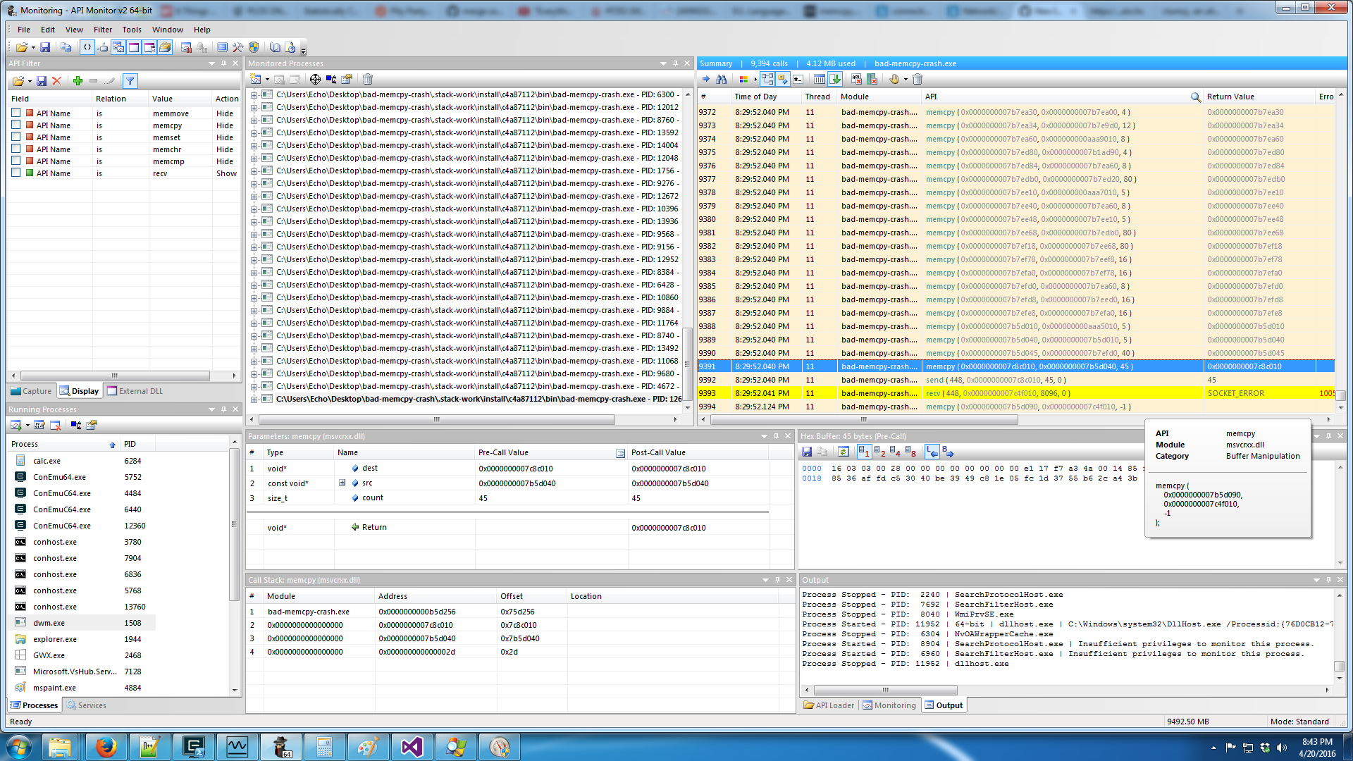
The most time-efficient tools were Clumsy and API Monitor. API Monitor lets you see every call to any Windows DLL. It clearly showed the failing call to recv followed by a memcpy with length -1 as well as repeated failing calls to send. It’s like a sort of super-strace in that it intercepts calls before a syscall is even issued. This is important since a lot of things that are syscalls on Linux are implemented in DLLs on Windows.
I also used hpc-strobe, a very cool and underappreciated tool. At regular intervals, it records a program coverage report. The trick is that these reports include counts of the number of times each expression was entered, not just booleans. You can take two reports, subtract one from the other and find out what code was executed in between the times it recorded them.
This was supposed to tell me what code it was hanging in. Unfortunately there’s a caveat I didn’t realize at the time: library code isn’t instrumented at all. Once it reported the hang happened while the socket handle was being evaluated, once while the hash of the download was being computed and once while parMapM_ was running. All of that was just coincidence: the hang wasn’t in any of the code that hpc-strobe can see. I did a lot of printf debugging trying to find the hang in places it wasn’t.
I still think it’s really cool, but knowing its limits is important.
I did a lot of printf debugging in the course of tracking down the bug. It was indispensable, but also tedious and error prone. An interactive debugger would’ve been great, but doesn’t really exist. GHCi’s debugger is better than nothing, but irrelevant in this case - it’s too different from how the program actually runs. In particular, it can’t use the threaded RTS so the bug doesn’t show up at all. You can load Haskell executables in GDB, but there aren’t any symbols in Haskell code and no backtraces either. There is preliminary work to improve the situation but it’s immature and as far as I can tell doesn’t work at all on Windows.
Conclusion
To save yourself tons of debugging time: question your assumptions and use powerful tools but know their limits. Printf debugging is useful but should only be used after you’ve exhausted the more efficient options.
Finally, I’m looking for programming work. If you or your company is looking for someone, particularly if the work involves programming language design and implementation, get in touch. It needs to be in Portland, remote, or cool enough that I’d want to move. My resume is here.
CommentsOne Week In
One week has passed since I resolved to work on four things one hour each, every day. I didn’t live up to the plan, but I got a lot more done on those four things than any week previously. I’ll call it a win. Categorized results:
Idris. This is less the Idris category and more the elaborate yak shaving necessary to do what I want to do with Idris. Before I started the “project”, I decided it would be good to land a tiny patch. I was going to bump some dependency versions, including zlib. It didn’t compile with the new version of zlib, because of some code that decompressed things and used Either to signal errors. That sort of thing should really live in the zlib bindings. So I wrote a patch against darcs zlib. The maintainer hasn’t responded to my email yet, and in the time since I started, Idris’ zlib dependency was dropped and replaced with zip. It was nice to finish something though, even if it didn’t actually matter much. Other users of the zlib bindings will hopefully benefit from my code.
After finishing that off, I started in on cabal bug 2614. The plan here is to use Cabal’s new custom-setup feature and Shake to improve Idris’ build system. Bug 2614 makes using custom-setup a little irritating. The fix is trivial, but breaks other things because of bug 1575. More work on that next week.
Games. I’m making a vignette game about how hard it can be to get out of bed and do anything when you’re depressed. Need to learn Blender so I can put together an environment.
Public good problem. I’ve learned a little Coq from these video tutorials. Having fun. Things often seem like a soup of symbols though. I know what they mean individually, but not together or their implications. The things I’ve done are all theorems in logic, so they’re extremely abstract.
Exercise. I’ve only done exercise on purpose once since last week :(. Try to do better this week.
More posts in the archives.